After reading this essay you will learn about:- 1. Introduction to Break Even Analysis 2. Assumptions Underlying Break Even Analysis 3. Applications 4. Non-Linear Break-Even Analysis 5. Limitations.
Essay # 1. Introduction to Break Even Analysis:
This is also known as cost analysis. Break even analysis is concerned with finding the point at which revenues and costs are exactly equal. This point is known as BREAK-EVEN-POINT. Thus this is a volume of output at which neither a profit is made nor a loss is incurred. Therefore production or sale must not be allowed to fall beyond this point. This analysis can be carried out either algebraically or graphically.
Break-Even Chart:
A breakeven chart is a graphical representation of the relationship between costs and revenue at a given time, and determines the break-even-point and profit potential under varying conditions of output and cost.
Functions of Breakeven Chart:
(i) To represent economical position of production on graph.
(ii) To for tell likely profits or losses at various levels of output.
(iii) To help the management to decide the production level.
(iv) To indicate margin of safety.
Essay # 2. Assumptions Underlying Break Even Analysis:
1. All the costs are either perfectly variable or absolutely fixed over the entire range of production.
2. All revenue is perfectly variable with the physical volume of production.
3. The volume of sales and the volume of production are equal.
4. In case of multi product firms, the product mix should be stable.
Essay # 3. Applications of Break Even Analysis:
Break even analysis not only highlights the areas of economic strength and weaknesses in the firm but also helps in finding out the ways which can enhance its profitability.
With the help of this analysis management of a production firm can take decisions related to the following:
(i) Safety margin. It decides the extent to which the firm can afford to decline in sales, before it starts incurring losses.
(ii) Volume needed to attain target profit. –
(iii) Change in price, and its effect.
(iv) Whether to expand production capacity or not.
(v) Whether to add a new product or drop production of any product.
(vi) Whether to make or buy.
(vii) Selection of production machinery so as to get maximum profit for a particular volume of the product out of the available machineries.
(viii) Improving profit performance by
(a) Increasing the volume of sales, and or
(b) Increasing the selling prices, and or
(c) Reducing the variable expenses per unit, and
(d) Reducing the fixed costs.
Example 2:
Fixed costs in a factory is Rs.10,000 per year, the variable costs are Rs.2.00 per unit and the selling price is Rs.4.00 per unit, calculate B.E.P.
Example 3:
If in example 1 sales are 8000 units, calculate safety margin. If desired profit is Rs. 6000, calculate target sales volume.
1. Safety Margin:
It refers the extent to which the concern can afford to decline in sales upto the break-even point. It can be represented by the percentage ratio of sales over break-even point volume to the sales volume.
... Safety margin = Sales volume – Sales at B.E.P./Sales volume × 100
2. Quantity Needed to have Desired Profit:
This is the most common application of break-even analysis and the desired quantity is given by
Target quantity = Fixed cost + Target profit/Contribution per unit
3. The Effect of Change in Price:
Sometimes management is required to consider whether to reduce price of a product or not.
Management has to consider the following facts in this regard:
If the sales price is reduced then contribution margin will reduce and this will increase the sales volume. But this increased volume may or may not receive increase in demand because it depends on elasticity of demand.
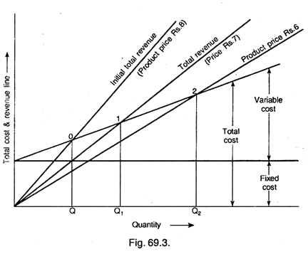
The change in break-even point due to rate variation in sales price is drawn below (Fig 69.3). At different price levels total revenue line can be plotted and the chart shows that as the price of a product is reduced the break-even point shifts towards right side and vice versa. From the chart, one can then estimate the volume that will be sold and profit at each price level.
From the chart
4. Effects of Change in Costs:
There are two types of costs:
(a) Variable cost, and
(b) Fixed cost.
(a) Variable Cost Change:
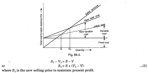
An increase in variable cost leads to reduction in the contribution margin. This increase in variable cost will reduce the profit. Therefore, what should be the new price to maintain the present profit without any change in sales volume.
As there is reduction in contribution margin, it will cause increase in sales volume. Therefore, what should be the sales volume to maintain the present profit without change in the price (Fig. 69.4).
Due to increase in the variable cost, Break-even point have shifted from point Q to point Thus higher quantity is to be sold to maintain the present profit assuming no change in the price of the product.
(b) Change in Fixed Cost:
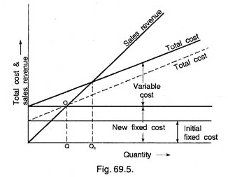
The fixed cost may change due to an increase in executive salaries, taxes, insurances and building rent etc. This is turn will bring change in the breakeven point, assuming no change in product price.
The Break-even point has shifted from point 0 to 1. If there is no change in price and volume of profit is maintained or there will be a rise in the sales price, if there is no change in the sales volume, provided profit is maintained.
5. Whether to Accept an Order or Not:
If extra capacity to produce a product is variable then sometimes management has to decide whether to accept another order at a price with less than the initial selling price. For example, a plant is operating on its 50% of full capacity. A buyer offered to buy 4000 units at Rs.5 per unit while the average cost is Rs.6. Now the problem is whether to accept this order or not.
The other details of the product are:
Total capacity = 20,000 units
Present output = 10,000 units
Direct material cost = Rs.10,000
Direct labour cost = Rs.10,000
Fixed costs = Rs.40,000
In this question, one can find that additional cost of making these 4000 units is Rs.4000 for material cost and Rs.4000 for labour cost (total Rs.8000) and the revenue from sales would be;
Rs.4000 × 5 = Rs.20,000
Thus the concern will save,
Rs.20,000 – Rs.8,000 = Rs.12,000
So, it would be profitable to accept anything more than Rs.2 per unit which is the direct cost per unit. There is only danger that, if other consumers come to know that this product is being sold at a lower price, they may also then demand supply at the lower price or otherwise they may not be further interested to buy from this concern. Therefore, in such cases acceptance should be kept secret.
6. Whether to Add or Drop a Product Line:
In this case, following two situations arise:
(a) Should a new product be added in view of the estimated revenue and cost?
(b) If the product is dropped from the line, what would be consequent effects on revenue and costs?
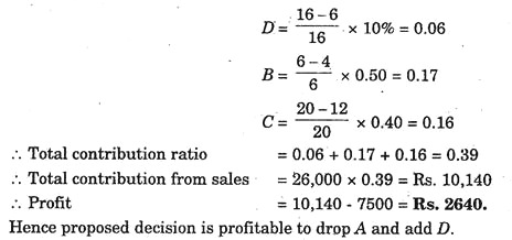
Example 4:
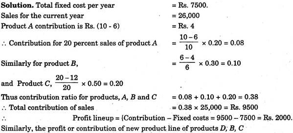
The following data from a plant is available:
Fixed cost per year = Rs.7,500
Total sales of three products = Rs.25,000
It is decided by the management to drop the product A and add product D. To find whether this decision is profitable or not?
Assume sales for products B, C and D as Rs.26,000.
Whether to Make or Buy:
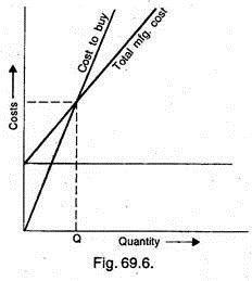
Assuming the cost to purchase is in direct proportion with the quantity purchased, the Break-even point can be plotted as shown in Fig. 69.6.
Let Q be the quantity at Break-even point, for less than Q it is cheaper to buy; and for more than Q it is cheaper to make.
It can also be written as,
Q = Fixed cost/Purchase price – Variable cost
Thus in this way Break Even Point theory can be applied to solve several problems of an industry such as minimum quantity to be manufactured to avoid losses, which machine will be profitable for a particular production etc. This theory is used as a tool by management to aid in making decisions.
Essay # 4. Non-Linear Break-Even Analysis:
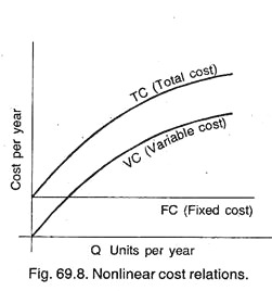
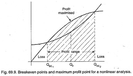
Till now, we have discussed linear break-even analysis, but in practice, some-times unit variable costs (V.C) decreases as the quantity level rises, this results total curve (TC) curve as a non-linear curve as shown below:
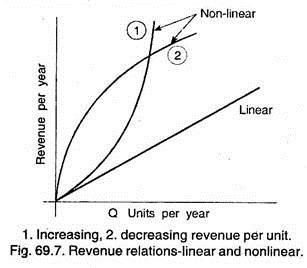
If nonlinear R (Revenue) or TC (Total cost) models are used, there may be more than one break-even point. Figure 69.9 presents this situation for two break-even points.
In this case, the maximum profit is obtained by operating at a quantity Qp, which occurs between the two break-even points and when the distance between the R and TC relations is greatest.
Break Even Analysis as a Tool for Decision-Making:
This analysis is used as a tool by management to aid in making decisions:
1. It can be applied to solve several problems of an industry such as minimum quantity to manufacture to avoid losses which machine will be profitable for a particular production etc.
2. It helps to determine the unit cost of a product, corresponding to any particular quantity of production.
3. It suggests about the selling price fixation.
4. It informs about the percentage financial yield for a project.
5. It informs about the fact that industry must run at its scheduled target capacity to get advantage of the optimal cost of production per unit.
Example 5:
(a) What is break-even analysis? What information does it provide to the management?
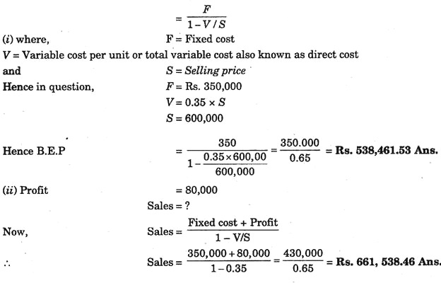
(b) The fixed costs of a company are Rs.350,000. The net sales amount to Rs.600,000 annually. The direct costs are 35% of sales in rupees.
Determine the following:
(i) The “break-even point” in terms of sales rupees,
(ii) The sales required to earn a profit of Rs.80,000.
Solution:
(a) Break-Even Analysis:
Equipment’s are used to produce products at profitable rate, so that the products can stand competition, replacement decision is not an easy job, it requires several consideration. As it involves large capital investment, hence a wrong decision may adversely effect the profitability of whole concern.
Therefore, a scientific approach to solve this problem is essential. For this purpose the theory of Break Even Point is very helpful. The break-even point of any two variable situations is the point or the value at which they become equal as the result of a common variable.
Let cost be the common variable in two situations 1 and 2, then cost equations will be
C1 = f1 (x) … a function of (x) …(1)
c2 = f2 (x)… another function of (x) …(2)
To solve for the value of x, let c1 = c2
i.e. f1(x) = f2(x) …(3)
Equation (3) can be solved for obtaining the value of (x). The value of x making the cost equal in both the situations is called “Break Even Value” (Fig. 69.1) Below the value of x, one situation will be economical while above it another situation will be economical.
(b) Break-Even Point, B.E.P.:
Example 6:
(a) What is meant by break-even analysis? Discuss the assumptions that underline the technique and its uses.
(b) In the past two years it is observed in metal working industry that the material cost has risen by 20% whereas other costs have risen by 10%. Assuming that the selling prices have advanced by 10% and that material costs represents 33 1/3 % of the total cost. Indicate the effect on the break-even point of typical break-even chart.
Solution:
(a) Break-Even Analysis:
A business is said to break even when its income equals expenditure. The break-even point means the level of output or sales at which no profit or loss is made. Below the Breakeven point, the loss occurs and above this point profit is earned.
The various assumptions that underline in this technique are given as under:
(i) It is assumed that over the entire range of volume of production all costs are perfectly variable.
(ii) It is assumed that over the entire range of volume of production all costs are absolutely fixed.
(iii) It is assumed that with the physical volume of production all revenue is perfectly variable.
(iv) The volume of sales and volume of production are equal.
(v) It is assumed that for multi-product firms, the product mix should be stable.
(b) Suppose initial total variable cost = Rs.300
Fixed cost will be same in all the conditions. Thus variable cost will be proportional to total cost. Now according to question after two years, material cost increases by 20% and other cost by 10% and material cost is 1/3 of total cost. It means if material cost is 100, other cost will be Rs.200. Thus total cost is Rs.100 + 200 = Rs.300.
New Material Cost = 100 × 1.20 = 120
New labour cost = 200 × 1.1 = 220
... New total variable cost = Rs.340
Let initial selling price = Rs.350 (we can assume any value)
After 2 years, new selling price = Rs.350 × 1.1 = Rs.385.
Output in both the situations is assumed to be any fixed quantity. Now if plot is drawn between total cost and selling price for the initial situation and new changed situation.
It is found that the Break-Even Point has shifted from right to left. It means new breakeven point will be at lower output and angle of incidence also large, which shows that profit margin is also more in the changed situation.
Example 7:
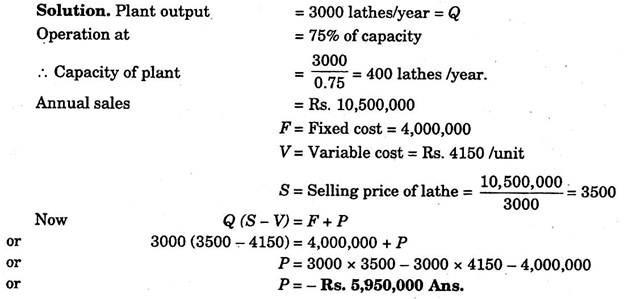
A plant is manufacturing 3000 heavy duty lathes per year and is operating at 75% of its capacity. The annual sales return is Rs.10,500,000. The fixed cost of the plant is Rs.4,000,000 and variable cost Rs.4150.00 per unit. There is a proposal to utilise spare capacity by manufacturing precision lathes which would increase the fixed cost by Rs.800,000 but reduce the variable cost by Rs.750 per unit.
(i) Is the proposal economical? Give reasons for answer.
(ii) If reduction in selling price by Rs.500 per unit requires the plant to run at 90% of its capacity to break-even, would this be a better proposal than the earlier one.
First Proposal:
Plant will use spare capacity in the manufacture of precision lathes.
Spare capacity = 1000 units
Here, Fixed cost F1 = 4,000,000 + 800,000 = 4,800,000
Variable cost V1 = 4150 – 750 = Rs.3400
Q1 = 3000 + 1000 = 4000 units.
Assuming sales price same, then
Q1(S – V1) = F1 + P
or 4000 (3500 – 3400) = 4,800,000 + P or P = – 4,400,000
Here again there is loss but this loss is less than the initial loss and this can be recovered by increasing the price of precision lathes (1000 lathes produced by utilising spare capacity). In calculations we assumed Rs.3500 per unit but being precision lathes, its selling price can be much higher.
Second Proposal:
Here we have to utilise 90% of the capacity at B.E.P.
In this proposal the loss will be extremely high. Therefore, it is not possible to accept this proposal. Hence first proposal should be accepted and loss may be recovered by keeping higher selling price of 1000 units of precision lathes.
Essay # 5. Limitations of Break-Even Analysis:
1. Since Break Even Analysis is based on accounting data therefore, it can be sound and useful only if the firm in question maintains a good accounting system.
2. It is based on the assumptions of given relationships between costs and revenues, on one hand, and input on the other.
3. Cost data’s of the past period may not hold good for the current period.
4. Selling costs may not remain constant.
5. The cost revenue-Volume relationship is linear. But this is realistic only over narrow ranges of output.
6. Break even analysis is not an effective tool for long range use and its use should be restored to the short run only.


