In this article we will discuss about:- 1. Introduction to Black-Scholes Model 2. Assumptions of Black-Scholes Model 3. Advantages 4. Limitations.
Introduction to Black-Scholes Model:
It is a tool for pricing equity options. Fischer Black, Myron Scholes and Robert Merton were awarded the Nobel Prize in Economics for developing this model in 1973. Prior to its development there was no standard way to price options.
As per the Black-Scholes Model, the fair value of a call option is a function of 5 key variables:
(a) Current value of share
(b) Strike price
(c) Time to expire
(d) Interest rate
(e) Volatility of price of underlying stock
Assumptions of Black-Scholes Model:
Assumptions of Black-Scholes Model are as follows:
(a) The price of the underlying stock moves randomly.
(b) Short selling of the underlying stock is possible
(c) Stock is being traded continuously
(d) There are no transaction costs or taxes
(e) All securities are perfectly divisible (e.g. it is possible to buy 1/100th of a share).
(f) The risk free interest rate is constant, and the same for all maturity dates.
(g) The call option is an European option
(h) There are no arbitrage opportunities.
(i) It is possible to borrow and lend cash at a constant risk-free interest rate,
(j) The stock returns are log-normally distributed.
A lognormal distribution is skewed to the right, which means it has a longer tail towards it right as compared with a normal distribution that is bell-shaped. The lognormal distribution allows for a stock price distribution of between zero and infinity and has an upward bias. This is because while a stock price can only drop 100%, it can rise by more than 100%.
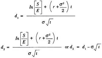
As per Black-Scholes Model,
Co = SN (d1) – Ee-rt N (d2)
Where,
Co = The equilibrium value of call option now (theoretical option price)
S = Stock price (price of underlying asset)
E = Exercise price (strike price)
e = 2.7183 = exponential constant (base of natural logarithm)
r = continuously compounding risk free rate of interest
t = time remaining until expiration (expressed in years)
N (d) = value of standard normal cumulative distribution function
In = Natural logarithm
σ = Standard deviation of the continuously compounded annual rate of return on stock. (Annual volatility of stock price)
Po = The equilibrium value of put option now (theoretical option price)
Black-Scholes model can be used for valuation of put option with the help of following formula:
Po =Ee-rt N (-d2)-SN (-d1)
Advantages of Black-Scholes Model:
i. It enables one to calculate a very large number of option prices in a very short time,
ii. It works entirely on objective figures rather than human judgment
Limitations of Black-Scholes Model:
i. Black-Scholes model cannot be used to accurately price options with an American-style exercise as it calculates the option price at expiration only. Early exercise as in the case of American option cannot be priced correctly using this model which is a major limitation of this model.
ii. All exchange traded equity options have American-style exercise as against the European options which can only be exercised at expiration. That means this model cannot be used for pricing most Exchange Traded options. The exception to this is an American call on a non-dividend paying asset as the call is always worth the same as its European equivalent since there is never any advantage in exercising early.
iii. It makes many assumptions which are not true in reality like it does not consider transaction costs, dividends on the underlying stock, etc.
Following are some of the terms which are commonly used in option trading:
(A) Delta (D):
It measures the change in option premium expected from a small change in the strike price, all other things being the same.
Where, “S is a small change in stock price and “C is the corresponding change in the call price (premium).
(A) Vega:
It is the rate of change of the value of the portfolio with respect to the volatility of the underlying asset. If Vega is high in absolute terms, volatility changes have relatively little impact on the value of that portfolio.
(B) Theta:
It is the rate of change of the value of the portfolio as time passes by with all else remaining the same.
(C) Gamma:
Gamma is the rate of change of the option’s Delta with respect to the price of the underlying asset. In other words, it is the second derivative of the option price with respect to price of the underlying asset.
(D) Rho:
The Rho of a portfolio of options is the rate of change of the value of the portfolio with respect to the interest rate. It measures the sensitivity of the value of a portfolio to interest rates.
