In this article we will discuss about:- 1. Concept of Simulation 2. Simulation Methodology 3. Procedural Steps in Simulation Analysis 4. Merits 5. Demerits 6. Models.
Concept of Simulation:
For many years, war games have been used as a means of training human resources and testing plans and equipment under field conditions.
The process of obtaining the essential qualities of reality without the reality itself is known as simulation. Simulation is the process of building, testing, and operating models of real-world phenomena through the use of mathematical relationships that exist among critical factors.
Simulation Methodology:
With the aid of high-speed computers, management can now simulate complex situations to determine the best course of action.
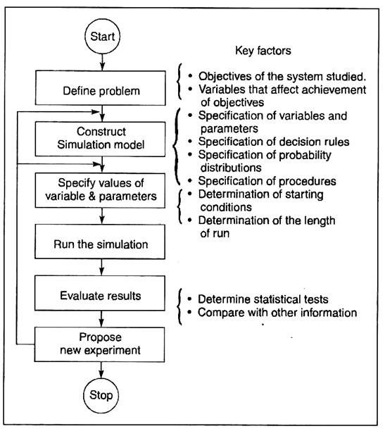
A typical simulation methodology is summarised in the diagram below:
Once a system has been designed, it can be simulated in a way that permits the system developer to test and refine the system. A business system is simulated by formulating a quantitative description or model of it. The model is then programmed for a computer, which can compress real-time and permit the effect of years of operations to be studied in a few minutes.
Through the use of simulation, management can study the effects of interrelationships of many variables (e.g., materials, money, information, manpower, and capital equipment) on organisational performance, thus allowing management to determine how a change in one variable will affect the other variables.
For example, an optimum inventory system may cause serious difficulties in the production department, so that the inventory system is best understood in the context of a simulation model which includes production, inventory, sales, and so on.
To cite another example, Airlines use computerised simulation models extensively to solve facilities and flight schedule planning problems. A computer simulation of airline systems is programmed to read raw schedule data including the type of aircraft and special factors affecting holding time, and to estimate delays and conflicts.
With such a simulation programme, the planner can study both proposed schedules and terminal layouts, test a variety of alternatives in a relatively short time, and develop an improved strategic plan.
Procedural Steps in Simulation Analysis:
In a simulation analysis, the following procedural steps are followed:
1. Model the project: The model describes how net present value is affected by the parameters and variables.
2. Specify the values of parameters and the probability distributions of the variables.
3. Select a value, at random, from the probability distributions of the variables.
4. Determine the net present value corresponding to the randomly generated values of variables and parameter values.
5. Repeat steps (3) and (4) in order to get a large number of simulated net present values.
6. Plot the net present values so simulated.
Merits of Simulation Analysis:
Simulation, as a tool of risk analysis, has the following merits:
1. Versatility of simulation technique helps in handling problems having a large number of variables—which would have been impossible otherwise.
2. A model, once built, can simplify the complex relationships existing among the parameters and variables concerning a project or problem.
3. Simulation technique assists the decision maker to explicitly consider the interdependencies and uncertainties concerning a project.
Demerits of Simulation Analysis:
Its demerits or limitations are:
1. Model building is a difficult task.
2. Specifying the values and probabilities is another hurdle.
3. An expert knowledge is essential for simulation application—which most decision makers do not possess.
Simulation Models:
The simulation techniques deal with outcome values for a strategy analyst. The models treat the behaviour of these outcome values—which a probability theorist calls a stochastic process. Strategic decision problems very closely resemble the known stochastic processes and are, therefore, readily simulated.
Markov Model:
This is alternatively termed as Markov Process or Markov Analysis.
To understand the basic nature of a Markov problem, let us consider the example below:
A major text book publisher stocks several thousand copies of a book. These books can be sold at retail price, sold at a discount, or scrapped because of obsolescence. These three outcomes are possible for each year the books are inventoried. The problem is: how many books can the publisher expect to sell at retail, sell at discount, or scrap each year of the inventory period?
A Markov process looks at the above example in terms of ‘states’ of outcomes.
The states are:
(i) Sale at retail price,
(ii) Sale at discount, or
(iii) Scrap during a given year of inventory.
This kind of analysis focuses on movement from state to the other state and from one time period to the next. Such movement is called ‘transition’.
The Markov model focuses on these transitions from state to state and evaluates the probability of each transition. In other words, the model estimates the probability of movement from one state to another and from one time period to the next. These probabilities are called ‘transition probabilities’ and are central to understanding the Markov process.
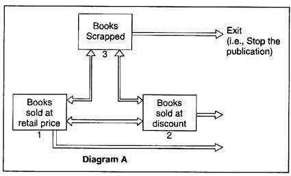
The Markov process may be illustrated in a diagram A below:
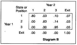
The ‘Matrix of Transition Probabilities’ (with hypothetical figures), given in diagram B below, represents what a Markov Analysis might find if we compare the position of ‘States’ in year 1 with those in year 2:
In diagram A, each ‘state’ is represented as a box. The lines connecting the boxes represent movement from one ‘state’ to another. The ‘states’ numbering 1 and 2 are possible moves. The ‘state’ numbered 3 represents a move towards exit; that is, the publication is stopped.
By reading across row 1 in the Matrix, for example, the strategy analyst can predict that 80% of the books will remain in position 1, 3 per cent will transfer to position 2 and 10 per cent to position 3.
To sum up the whole issue, we can say that Markov analysis helps in:
(i) Predicting market share, in terms of sales, of a product on a future period,
(ii) Predicting a steady future market share in terms of sales, and
(iii) Studying the future course of action in terms of a suitable strategy.
In essence, the Markov analysis provides management with some idea of the behaviour of consumers in terms of their loyalty to brands and their switches from brand to another.
Queuing Models:
Queuing models are also known as waiting line models. In both production and service systems, waiting lines are found. People wait for banking services. Parts and accessories and components queue up for their turn in a machine or assembly shop and waiting time in the process is variable.
Because such waiting lines affect both the service process and the customer, the operations manager must look at operating costs, efficiency and customer satisfaction.
The problem here, in its simplest form, is a trade-off—the cost of keeping a customer waiting on one hand, and the cost of idle services on the other.
For example, an aircraft’s time in the air and also on the ground is very costly. Due to this, the airlines ask the customer-passengers to come to airports early so that flight schedules can be maintained, apart from check-in formalities. Computer simulation in this problem area is an example of queuing or waiting line model, and the programme is termed QUESIM. This technique is called Monte Carlo Simulation.
Decision Tree Model:
A probabilistic model which is used for planning is the Decision Tree.
The Cost-Volume-Profit analysis and Linear Programming techniques can clarify the value of any particular decision, given the assumption of certainty about outcomes.
But when several choices of products are available for capital investment, or when several combinations of products may be scheduled within given operational capacity, a systematic and quantifiable approach to choosing among alternatives is called for. Often a decision tree is used for this purpose.
In short, Decision Tree model is appropriate when a series of decisions must be made but the outcome of each is unknown.
Illustration:
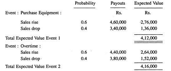
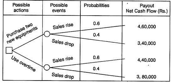
Let us consider that a medium-sized electronics component manufacturer has to make a decision about purchasing some new equipment or meeting rising sales with overtime production. Management could identify the alternatives, their costs, and the subjective probabilities of occurrence as shown below (hypothetical);
It becomes clear that the best decision is to operate at overtime.
A decision tree model will appear like:
In this particular case, the odds and pay-outs were extended one year longer and it was found that on a two-year or longer payout (more futurity) the new equipment would be a superior choice.
Although the decision tree does not provide a definitive answer, it does clarify the strategist’s thinking. Such trees are particularly useful to examine the risks and rewards of proposed projects and achieve consensus among top-level decision groups.
DECIDE is a computer programme, used in decision tree analysis. DECIDE documentation includes an example of a decision tree, and the needed probability, costs/benefits, and other inputs, as well as how to adjust future cash flows using present value and probability models.
