This article throws light upon the top six methods used in operation research. The methods are: 1. Linear Programming 2. Transportation Problems 3. Waiting Line or Queuing Theory 4. Game Theory 5. Simulation and Monte Carlo Technique 6. Dynamic Programming.
Method # 1. Linear Programming:
Linear Programming is a mathematical technique for finding the best use of limited resources of a concern. This is a technique to allocate scarce available resources under conditions of certainty in an optimum manner.
By using linear programming technique, a production manager can allocate the limited amount of machine time, labour hours and raw material available with him to the different activities so as to maximise the output/profit.
For solving a problem by linear programming, following conditions must be fulfilled:
i. Objective i.e., reduction in cost or to maximise the profit, be stated mathematically.
ii. Resources can be measured as quantities i.e., in number, weight, volume or Rupees etc.
iii. There may be many alternative solutions.
iv. Relationship between factors should be linear.
v. Restrictions of the resources must be fully spelt out.
Methods:
There are several methods to solve linear programming problems such as graphical, index distribution, simplex and modified distribution (MODI) methods. But the graphical method is quite easy and simple. The other method commonly used is simplex method.
A. Graphical Method:
To understand graphical method, let us take following example:
Example 1:
Objective of a firm is to maximise profit by producing product A and / or product B both, of which have to be processed on machines 1 and 2. Product A requires 2 hours on both machines 1 end 2, while product B needs 3 hours on machine 1 and only 1 hour on machine 2. There are only 12 and 8 hours available on machine 1 and 2 respectively. The profit per unit is estimated at Rs. 600 and Rs. 700 in case of A and B respectively. Find out number of units of product A and B, he should produce to maximise the profit?
Solution:
First Step:
Formulation of Linear programming problems. Let Z is the profit. The maximum profit by manufacturing A and B.
600 A + 700 B = Max. profit Z …(1)
This equation is called objective function.
Now set up the equations for the process times.
Machine I – 2A + 3B ≤ 12 …(2)
Machine II – 2A + B ≤ 8 …(3)
Second Step:
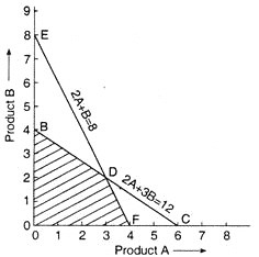
Plotting of the equations on graph (Fig. 30.1). Suppose product A is shown on X-axis and product B is shown on the Y-axis of the graph. Now to plot the equation 2A + 3B ≤ 12>, first find the two terminal points, and then joining these points by a straight line.
Now the question is how to find the two terminal points:
(a) Suppose all the time available on machine 1 is used for making product A, this means the production of product B is zero, this means 6 units of product A would be made, then the first terminal point is (6, 0).
(b) Now supposing that all the time available on machine 1 is utilised for making product B then the production of product A is zero, and only 4 units of product B would be made. The second terminal point is (0, 4).
By joining (6, 0) and (0, 4), we get a straight line BC.
In the same way, the other equation 2A + B ≤ 8 can also be drawn by a line EF by terminal points (4, 0) and (0, 8).
Third Step:
Identify Feasibility Region and ascertain co-ordinates of its corner points. Under this step we have to identify the cross shaded area BOFD (Fig. 30.1), generally known as Feasibility Region and then finding on the co-ordinates of its corner points. These co-ordinates can directly be read with the help of accurately drawn graph or we can also find the co-ordinate with the help of mathematics such as;
O (0, 0)
B (0, 4)
F (4, 0)
and for point D, solve the two equations
2A + 3B = 12
2A + B = 8
On solving, we get A = 3, B = 2, so the co-ordinate of point D is (3, 2).
Fourth Step:
Test which corner point is most profitable. Putting different co-ordinates of corner points in the objective function Eq. (1), amount of profit in hundred Rupees.
Corner point O (0, 0) = (6 × 0) + (7 × 0) = 0
Corner point B (0, 5) = (6 × 0) + (4 × 4) = 16
Corner point F (4, 0) = (6 × 4) + (7 × 0) = 24
Corner point D (3, 2) = (6 × 3) + (7 × 2) = 32
Thus corner point D is yielding maximum profit of Rs. 3200 and the firm must produce 3 units of product A, and 2 units of product B.
B. Simplex Method:
To solve the linear programming problem, simplex method is quite common. There are several ways to solve the problems by simplex method, but the most easy one is with the help of “Gauss-Jorden reduction process”.
Let us first understand the Clauss Jordan reduction process with the help of following example:
Example 2:
Let the following three equations are in five unknown, find solution for C, D, E in terms of A and B.
2A – B + 2C – D + 3E = 14
A + 2B + 3C + D = 5
A – 2C – 2E = -10
Solution:
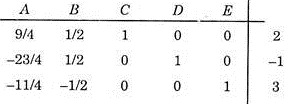
Let us rewrite the given equations in the matrix form.
Now our aim is to eliminate C from all equations except the first, D from all equations except second, E from all equations except third, so that in the final set of equations, there must be unit coefficients in place of variables.
This can be done with the help of steps I, II and III described as under:
Step I:
Divide each entry in the first row by 2, coefficient of C in the first equation. Coefficient of C (i.e., 2) is called pivot and is circled in the first matrix, this causes the coefficient of C equal to unity.
Step II:
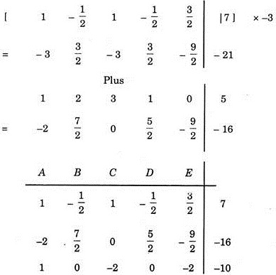
Now multiply the new first row by negative coefficient of second row against C (i.e. by -3) and add the result with the second row.
Step III:
In the same way, multiply the new first row with (+2) and add the resultant with third row.
Thus the final matrix will be:
In the same way, eliminate coefficient of D except second equation.
Step I:
Divide second row by 5/2, we get
Step II:
Multiply new second row by — and add the resultant with 1st row
Step III:
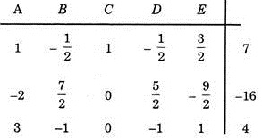
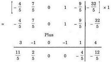
Multiply new second row by 1 and add the resultant with third row we get
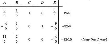
Thus the final matrix will be
In the same way, eliminate the coefficient of E from all equations except the third by repeating the procedure
Divide new third row by -4/5, we get
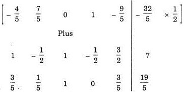
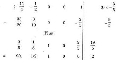
Now multiply the new third row by negative coefficient of first row against E (i.e. by -3/5) and add the result in the first row
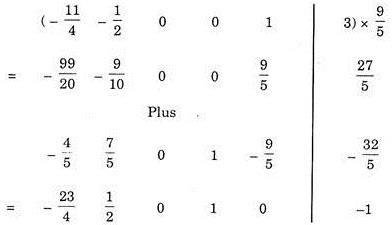
Now multiply the new third row by the coefficient of 2nd row against E (i.e. by 9/5) and add the result with second
Thus the final matrix equation will be
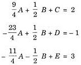
Thus we can rewrite the three equations as follows:
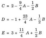
Thus the answer will be
Further C, D and E are known as basic variables and A and B as non-basic variables. If non- basic variables are zero, then the solution obtained is known as “Basic solution”.
Thus in this example, the basic solution is:
C = 2, D = – 1 and E = 3
It may be added that we can choose any number of basic variables and obtain the basic solution.
On observing, we see that to get a basic solution, it is not necessary to work out the operation on the coefficients of A and B at each step, since we intend finally to equalise them to zero.
Method # 2. Transportation Problems:
When a company have different manufacturing plants at different places, and have different sites for further distribution of products, we face a problem because if the production capacities of plants are different then it is not possible to ship all the different requirements from the nearest plant.
When this happens, the question immediately arises as to which is the most economical shipment of product from different plants to the different sites. To solve such problem ‘operation research’ helps, which involves a mathematical technique called ‘Transportation model’.
Example 3:
Let there be three plants A, B and C and three sites 1, 2 and 3. These capacities and requirements are as per Table 1.
The transportation costs in Rupees from plants to warehouses are shown in Table 2.
There is no other condition; any plant can transport the product to any site up to its requirement. Now the problem is to find most economical shipment, i.e., to minimise the total transportation costs.
First prepare a table showing the requirements and capacities of sites and plants respectively. This type of table is known as Matrix. (See Table 3).
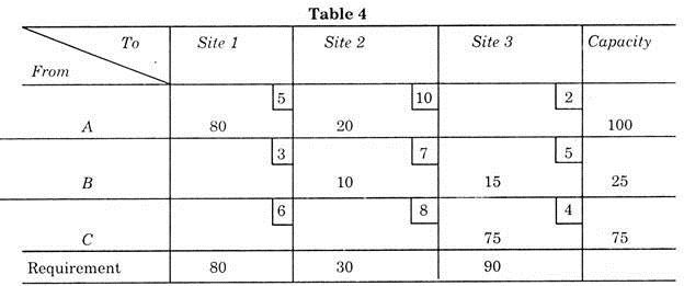
Now put the transport cost at the small square at right corner of large square, as shown in table 4 and apply the northwest corner method (but remember that it is not necessary to solve the problem by this method but for systematic approach this is helpful).
Using this north-west corner method, in the west corner square put the smaller of the two values between the capacity and requirement for the required column. As per example, we have two values 100 and 80, thus putting 80, in the corner as shown in Table 4. This means that transport 80 parts from plant A to site 1. This will fulfill the requirement of site 1, but the entire capacity of plant A is not utilized. Before proceeding to plant B, the remaining capacity of plant A must be utilized.
To do this, place 20 parts still available under site 2 which needs 30 parts. This utilizes the plant A capacity, so now move to plant B. As already 20 parts are shipped to site 2, only 10 parts are needed. These parts may be transported from plant B. Now for site 3, we first ship the remaining capacity (25 – 10 = 15) of plant B and remaining needed by site 3 from point C.
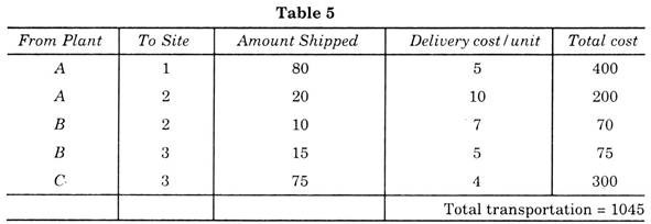
This solution of problem now known is called “initial solution” because it is not possible to say that this distribution is most economical. Total transportation cost is now computed as per Table 5.
The next step is to know whether this solution is the best one i.e. whether the transportation cost cannot further reduce.
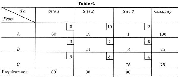
To do this, transfer-one part from plant A to site 3. Now balance the Table 4, and only 19 parts are to be shipped to site 2.
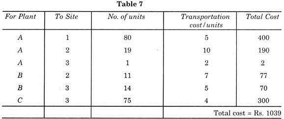
Now for this solution, cost table is computed as per Table 7.
Now this shows that solution in Table 7 is more economical than the initial solution which causes a saving of rupees (1045 – 1039 = Rs. 6).
To get the final solution of problem, repetition of the above process of moving one unit from one centre to another at a time until optimal solution is found. This type of method requires much labour. Thus to avoid this cumbersome method, another method is utilised to get final solution with less labour. This method is known as ‘Stepping-stone’ method.
Stepping-Stone Method:
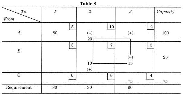
Refer Table 4 to select a square which is empty. Starting from the square under site 3 and opposite Plant A, let us call 3 A square. Next trace a closed loop path from this empty square moving horizontally and vertically only back to this empty square.
Put the positive sign in the starting square 3A and to 2A square giving it a minus sign. Next we move 2B giving positive sign then to 3B which minus sign, then back to 3A. Table 8 shows this path on the original Table 4 with signs.
By applying this plus and minus values in this dosed loop path to the transportation cost in each square we get the amount of improvement by shifting one unit of production from SB to 3A and so on. As we started from 3A, square, let this path be known as 3A path. Thus the saving is given by due to this = 3A – 2A + 2B – SB, substituting the value from right hand corner of each square.
3A path = 2-10 + 7- 5 = – Rs. 6
This shows that each unit from Plant A to site 3 have a saving of Rs. 6 which is similar to the result obtained by north-west corner method, i.e., Rs. 1045 – 1039 = Rs. 6.
After this, all the possible closed loops are found and calculations are done, as shown in Table 8(a).
From the above table, it is clear that only 3 A path is suitable because only in this path there is reduction in the transportation cost (because minus sign is obtained in the result). All other paths cause an increase in the cost.
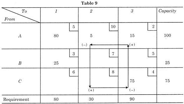
By trying to transfer maximum 15 parts from SB to 3A (least number of parts having minus square). Now Table 8 is changed to new Table 9.
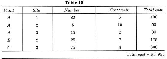
Now computing shipping cost as per Table 10.
This shows a reduction in the cost. Now again we choose another unused paths from Table 9.
There are two paths:
2C = 2C – 3C + 3A – 2A = 8 – 4 + 2 – 10 = Rs. – 4
C = C – 3C + 3A – 1A = 6 – 4 + 2 – 5 = Re. -1.
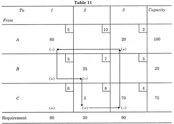
This shows that in both paths, there is reduction in cost, but to gain maximum, the higher negative value path is chosen. Then Table 9 changes to Table 11.
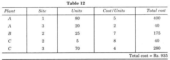
In this Table, we shifted 5 parts from 2 A because 5 is the least value in negative squares. Now shipping cost is as per Table 12.
Thus there is further reduction in the transportation cost. But this is not the final solution.
Analysing the solution of Table 11 by loop method, the paths are:
1B = 1B – 2B + 2C – 3C + 3A – 1A = 3 – 7 + 8 – 4 + 2 – 5 = Rs. -3
1C = 1C – 3C + 3A – 1A = 6 – 4 + 2 – 5 = Re. – 1.
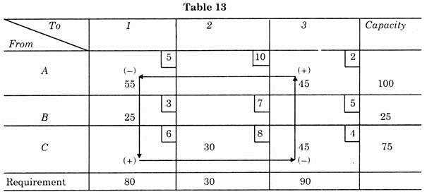
Thus 1B path is more economical. Shifting 25 parts (least value in negative squares), the new solution is shown in Table 13.
The transportation cost will be according to Table 14.
Thus a further reduction is there in the transportation cost. But to get optimal solution we have to test new unused paths.
1C = 1C – 3C + 3A – 1A = 6 – 4 + 2 – 5 = Rs. – 1
2A = 2A – 2C + 3C – 3C – 3A = 10 – 8 + 4 – 2 = Rs. 4
3B = 3B – 3A + 1A – 1B = 5 – 2 + 5 – 3 = Rs. 5
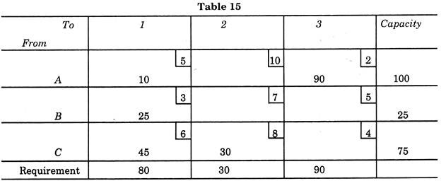
Thus a further improvement is possible by adopting path 1C. Transferring 45 parts (least value in negative square), the solution is as per Table 15.
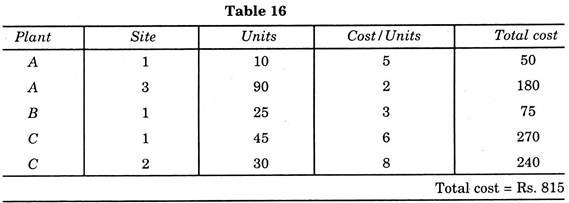
The transportation cost is calculated in Table 16.
Now to improve the solution further we have paths:
3C = 3C – 3A + 1A – 1C = 4 – 2 + 5 – 6 = Re. 1
2A = 2A – 1A + 1C – 2C = 10 – 5 + 6 – 8 = Rs. 3
3A = 2B – 3A + 1A – 1B = 5 – 2 + 5 – 3 = Rs. 5
2B = 2B – 1B + 1C – 2C = 7 – 3 + 6 – 8 = Rs. 2.
We have seen that all possible paths give positive values. Thus the solution of Table 16 is a final result, as now it is not possible to further improve that result, this solution is optimal solution.
Though this method looks a lengthy one, yet by doing this a saving of Rs. 320 (Rs. 1045 – Rs. 815) is realized with the help of operation research over the initial solution of Table 4.
Method # 3. Waiting Line or Queuing Theory:
The object of queuing theory is to examine the problem of waiting and minimise the waiting period or in other words by solving such waiting line problems, we can adjust the waiting time or can reduce the queue to have economical balance between the costs of equipment or people standing idle and cost of providing better service.
The theory can be applied wherever queues are visible may it be bank or post office counter, rail or airline booking window, raw material or semi-finished product waiting for next operation on shop floor or material waiting for inspection or for moving to another place or turner waiting for getting tools for tool room or vehicle waiting for its turn on a petrol pump or service station. Such delays add to the production cost or cause inconvenience during service.
Waiting line or queuing theory is used to solve queue formation situations by analysing the feasibility of adding facilities (manpower or equipment) and assessing the amount and cost of waiting time. This theory helps in determining the optimum amount of facilities (manpower, equipment etc.).
Assumptions in Queuing Theory:
i. The principle of first come, first served is followed.
ii. Length of queue i.e., number of items in the queue remains the same with the passage of time.
iii. Number of items in the queue as well as waiting time by a particular item is random variables, and is not functionally dependent on time.
iv. Arrival rates follow Poisson distribution and service times follow exponential distribution.
Applications:
Waiting line theory can be used for efficient decision making in the following fields:
i. To find optimum number of tool crib clerks.
ii. Selection of material handling equipment.
iii. Selection of the size of maintenance crew.
iv. Distribution of service facilities like rest room, first aid centres, drinking water booths etc.
v. Machine interference problem to find out the work load of a single repair man.
vi. Traffic congestion studies.
vii. Job shop scheduling.
viii. Matching construction equipment capacities e.g., Loading of dump trucks by a shovel, pusher dozer feeding a scraper, feeding a crushing plant, asphalt plant hopper by a dumper or a wheel loader.
The method can also be applied to other similar problems, where a team work of equipment is involved.
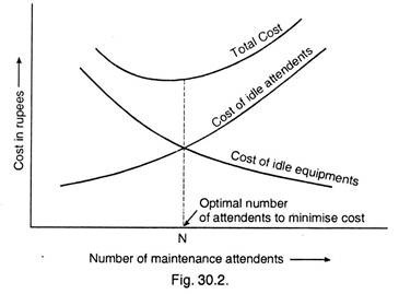
Let us take a waiting line problem. The main problem of waiting line generally occurs in maintenance department, where there is always a formation of queues because by nature the maintenance operation is an inefficient operation. To avoid the waiting line, if we employ many attendants then cost of keeping them is expensive, if we have few, then cost of idle equipment’s is again considerable.
This can easily be judged from Fig. 30.2.
If in a firm from the past records, it is found that 50 machines are to be repaired per day, but the problem is that how many attendants must be employed in the maintenance department economically.
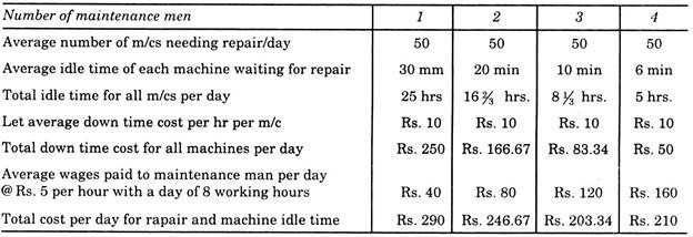
An analysis is done by finding the cost and idle times when 1, 2, 3, 4 attendants are employed, the computation is as follows:
Now looking at the above solution with all cost considerations, it will be most economical for the firm to employ three maintenance men.
Example 4:
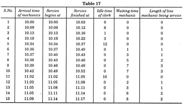
Let us assume that 12 mechanics at an average arrive at random per hour, i.e., one each in 5 minutes. The clerk can deliver the special tools after checking in 3 minutes. Table 17 gives a record of the servicing 15 mechanics. The average interval between arrivals is slightly less than 5 minutes.
Solution:
Clerk’s idle time = 32 minutes
Mechanics’ waiting time = 39 minutes.
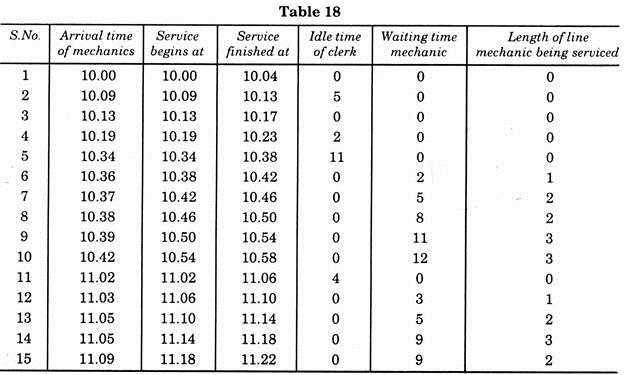
We see that for this problem, the clerk had 32 minutes idle time and the various mechanics waited for total 39 minutes. Now change the service time from 3 to 4 minutes. Now the Table 18 gives the schedule of servicing.
Clerk’s idle time = 22 minutes
Mechanics’ waiting time= 64 minutes.
This results in less idle time for clerk, but the waiting time for the mechanics is almost twice of that of previous one. Further we see that by increasing the service time, the waiting time and length of waiting line increase manifold. If the rate of arrivals is equal to the service time then we can assume that the waiting time and length of waiting line will increase and become infinitely as calculated latter.
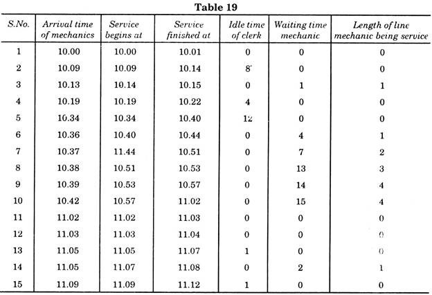
Now to have more realistic problem, let us assume that the service time is also random, and that the service time may also vary, depending upon the number of tools to be delivered, their sizes, weights and locations. Table 19 shows a record in this situation.
Clerk’s idle time = 26 minutes
Mechanics’ waiting time = 56 minutes.
On analysing above table, the clerk’s idle time and mechanics’ waiting time will depend on how the arrivals of mechanics’ will match up with the length of service timings. In general, mechanic arrives almost simultaneously with the request of requirements of long service times, and then waiting line will be relatively longer, while clerk is continuously busy.
Thus waiting time can forecast the probable waiting time and probable length of the line, and by this management can decide, what is optimum allocation of personnel and equipment to minimise cost. To do this, the nature of the distribution of arrivals and the service times must be known.
From Table 19 we can calculate, supposing that the clerk is paid at the rate of Rs. 2 per hour and he works for 8 hours per days, then
Cost of clerk’s idle time = 26/60 × 2 roman Re 0.87
This cost is for only 72 minutes, i.e., for 11.00 to 11.12 O’clock. Then cost of idle time/day
= 480/72 × 0.87 = Rs.5.80 per day.
Suppose the mechanic’s average wages are Rs. 3 50 per hour, then
Cost of mechanic’s idle time = 56/60 × 3.50 = Rs. 3.27 for 72 minutes.
Cost of mechanic’s idle time/day = 480/72 × 3.50 = Rs. 21.80 per day.
Thus total cost of idle waiting time = Rs. 21.80 + 5.80 = Rs. 27.60/day.
Now the problem is—would it be economical to have a second clerk? If the second clerk is to be added, then mechanics waiting time can be reduced, but total idle time for clerks would increased. If the net effect on the cost of idle plus waiting time is negative, the second clerk would be needed.
Mathematical Method:
In table 17, 18 and 19, we have explained simple waiting problem. With the use of mathematical formulae, we can directly get the data, in which we are interested, such as average length of waiting line and average waiting time, etc.
For solving queuing problems mathematically, an expression known as traffic Intensity is used. This is denoted by a letter ‘T’. This is the demand divided by the capacity or more clearly— the mean service time divided by the mean interval between successive arrivals.
The calculation of traffic intensity for any system is shown below:
Suppose the arrival intervals are:
5, 4, 10, 6, 3, 2, 6, 4, 8, 15, 2, 5, 4, 6, 8, 7, 3, 5, 2, 5, 8, 7, 4, 3, 2, 6, 7, 4, 3, 4, 7, 5, 8, 4.
The cumulative totals, obtained by adding the first to intervals and then the first three and so on, are:
9, 19, 25, 28, 30, 36, 40, 48, 63, 65, 70, 74, 80, 88, 95, 98, 103, 105, 111, 119, 126, 130, 133, 135, 141, 148, 153, 165, 160, 166, 171, 179 and 183.
Now cumulative averages obtained by dividing all the cumulative totals by the number of intervals making up each total are as follows:
9/2, 19/3, 25/4, 28/5, 30/6, 36/7, 40/8, 48/9, 63/10, 63/11
70/12, 74/13, 80/14, 88/15, 95/16, 98/17, 103/18, 105/19, 111/20, 119/21
126/22, 130/23, 133/24, 135/25, 141/26, 148/27, 153/28, 158/29, 160/30
166/ 171/179/ and 183/34 or in decimal
4.5, 6.3, 6.2, 5.6, 5.0, 5.1, 5.0, 5.3, 6.3, 5.9, 5.8, 5.7, 5.7, 5.9, 5.9, 5.8, 5.7, 5.5, 5.6, 5.7, 5.7, 5.5, 5.4, 5.4, 5.5, 5.5, 5.4, 5.3, 5.3, 5.3, 5.3, 5.4, 5.4.
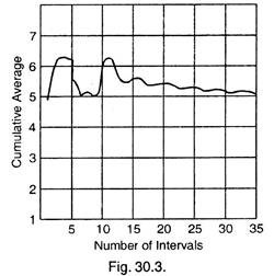
When these cumulative averages are plotted against the number of intervals, the curve will be as of Fig. 30.3. It shows that the curve fluctuates a little at the beginning, but then settles down to fairly steady figure of 5.4 minutes. Thus this value is taken as the average interval between arrivals.
The average service time also can be found in a similar way. Let us assume that it will be 4.5 minutes. Then the traffic intensity would be
Traffic intensity T = 4.5/5.4 = 0.833 ... T = A/S
where A = average arrival rate and S = roman the service rate.
Thus one waiting line serviced by one individual.
1. Mean number in waiting line, i.e. average length of waiting line (La)
= T2/1 – T = A2/S(S-A)
2. Mean or average number in line, including the one being serviced (L)
= La + A/S = A/1 – T = A/S – A
3. Average waiting time of an arrival
Wa = La/A = T/S(1 – T) = A/S(S – A)
4. Average time which an arrival spends in the system or say mean time in system including service
= W = L/A = 1/S – A = 1/S(1 – T)
5. Idle time = (1 – T) = idle time of service man.
In the Table 19, we have come across a distribution with Random Arrival time of mechanics and Random Service Time. With average arrival rate (A) as 12 per hour and average service rate (S) as 20 per hour, thus calculating as per given formulae.
A = 12 and S = 20
T = 12/20 = 0.6
Average length of waiting line La = T2/1 – T = 0.36/1 – 0.6 – 0.36/0.4 = 0.9
Average number in line, including the one being serviced
L = T/1 – T = 0.6/1 – 0.6 – 6/4 = 1.5
Average waiting time of an arrival Wa = T/S(1 – T) = 0.6/20(1 – 0.6) – 6/20 × 4
= 3/40 = 0.075 hr. = 4.5 minutes.
Average time which an arrival spend in the system
= 1/S(1 – T) = 1/20 × 0.4 = 1/8 hour
Idle time = (1 – T) = 40% of total attended time = 72 × 0.4 = 28.8 roman minutes.
The data computed above are approximately equal to the same value obtained from the simple simulation done in Table 19. The more correct and nearer value can be obtained by simulating average sample.
Probability that queue size exceeds n = (A/s)n
Probability that queue size is zero = 1-(A/S)/1-(A/S)c+1
where C = limiting capacity
when a man has to pass through more than one queue.
This means when a service is completed in phases and at each phase queue is available.
In such cases, following formulae are used:
(i) Average waiting time = (K +1) (A/S)/2KS (1 – [A /S])
(ii) Average queue length = (K + 1) (A/S)2/2KS (1 – [A /S])
Method # 4. Game Theory:
Suppose, a manufacturer who is faced with the problem of choosing a price for his product has the necessity to examine the reaction of his competitors, due to this decision about the price. Suppose, he is trying to decide whether it is worthwhile for him to cut his price, the answer will depend on what his opponent manufacturer will do.
There are four possible outcomes:
1. He cuts the price; the opponent keeps his price constant.
2. He cuts the price; the opponent also cuts the price.
3. He keeps his prices constant, the opponent cuts his price.
4. He keeps his price constant; the opponent keeps the ‘price’ constant.
Thus the manufacturer has to analyse all these different outcomes with the help of game theory which shows the profitability under each situation from which the manufacturer can make a final choice.
In game theory, the decision makers are known as ‘players’, the choices are called strategies and the preferences of the decision makers called “payoffs”.
If the sum of payoff is zero, the same is said to be zero sum, but where the sum of payoff is not zero, these are called ‘non-zero sum game’.
The game theory is a technique which introduces a table known as ‘payoffs matrix’, showing the expected values for various outcomes to determine the best way to ‘play’ against the opponent. The object is not to find the best answer, but to minimise the maximum (known as minimax) risk, or reduce your chance of losing.
The use of a ‘pay-off-matrix’ for expressing the problem and evaluating various decisions can have important implications for business or industries. But to make theory really practicable, the analyser should have lot of imagination and know new development of the science.
The theory can easily be more understandable with the help of following examples:
Example 5:
Consider the following table:
Solution:
The choices α, β, ү, δ are the possible strategies, for you and A, B, C, D are the possible strategies of your opponent. How should you play the game? If you play strategy β, you gain 2 points, if the opponent plays A or C, but lose 4 if he plays B. You cannot be sure when you play β what choice your opponent has made.
Here, a minimax rule exists. If you play strategy α, you win a minimum 2. If you play any other strategy, one might not win as much. If the opponent plays B, he does not lose more than 2. If he plays any other strategy, he could lose more.
Thus yours own minimum again is the same as the opponent’s maximum loss. The square αB is unique in this respect and is called the saddle point or the solution of the game when playing against a skillful opponent in the kind of situation one cannot do better in the long run than play this optimum strategy.
Example 6:
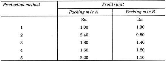
Suppose we are setting a plant to produce a new product. We have five alternative methods of manufacturing from which selection may be done. But profit depends on one of the experimental automatic packing systems which will be successful. There are 50-50 chances that either one or the other will be successful but definitely not both.
Depending on which one is successful to prepare the matrix for the five methods. The main problem is that we have to select and start installing the method of manufacture before we know which packing system will work about. So which method will be selected to assure the firm maximum profit?
Solution:
The answer is simple, we select method 3, because it assures us the greatest profit, in case machine B is successful and even we can earn, more in comparison of machine B, if the machine A is successful.
In game theory usually we assume that the opponent has perfect intelligence and always plays his best strategy to make us loose. There is our example, we are really playing against nature (such problems come under the games against nature) where opponent is nature which is trying to win with perfect intelligence, the nature will certainly pick machine B.
But this is unrealistic, because in competitive situations we take advantage of the fact that our opponent does not have perfect intelligence. This improves our chances of earning more profit; we can easily introduce more probabilities of each outcome to defeat our opponent.
Two Person Zero Sum Game:
This type of game can easily be understandable with the help of following example:
Example 7:
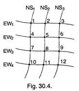
Let two candidates of different political parties say Congress and BJP have agreed to hold public meetings somewhere in their constituencies and are negotiating over the location.
Each wishes to have as friendly audience as possible, and the 12 possible locations vary considerably in the balance between Congress and BJP. Each of the 12 possible sites lies on the intersection of an east-west and a north- south highway, as shown in Fig. 30.4.
Solution:
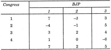
The audience advantage of Congress over BJP as east-west and north-south intersection is given in the form of matrix.
The Congress candidates now studies the matrix and tries to find that what is the worth that can happen to him if he chooses any route.
If he chooses I route, and thinks that if BJP candidate chooses route I or III then he has an advantage of 7 or 3 respectively, however, if worst is when the BJP candidate chooses route 2 then the loss is of 3.
Thus he writes -3 at the end of first row, and, similarly, copies the smallest minimum entry of each row at its end.
Now the strategy would be to choose route 3, which guarantees him an advantage of minimum of 2. This is called maximum strategy.
In the same way, the BJP candidate looks for the largest entry in which column (largest because his interest is exactly opposite those of Congress candidate) and chooses the column with the smallest maximum strategy.
Thus most advantageous route is 2 with minimum of column maxima = 2
Thus maximum = minimax = 2-, the solution here is clear one.
When the guaranteed minimum and maximum payoffs for two opponents are exactly equal (as in the above example), the game is said to have a Saddle Point. The presence of saddle point means, each player has nothing to gain by leaving the strategy which leads to the saddle point. A saddle point can be recognised by the fact that it is the smallest number in its row and the largest in its column.
Zero Sum Game without Saddle Point:
Suppose a game with matrix ![]() and have no saddle point, this can only be possible when b > d and c < d. Let the number matrix is as follows:
and have no saddle point, this can only be possible when b > d and c < d. Let the number matrix is as follows:
The maximum = 5 and minimax = 4 hence there is no saddle point. Thus to solve such problem, we employ a mixed strategy. To play the game, we have to find the probability.
According to the theory of probability, if Sohan chooses strategy 2 with probability p and strategy 1 with probability 1-pen when Mohan choose strategy 1, Sohan’s advantage is
Y1 = 3(1 – p) + 5p
when Mohan chooses strategy 2, Sohan’s advantage is
Y2 = 6 (1 – p) + 4p.
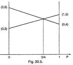
Now we want to choose p so that and y2 are both as big as possible. This will maximize the total expectation. Graphically, we find that this point is at the intersection of the two lines and occurs (Fig. 30.5) when
p = 3/4 and (1 – p) = 1/4 and y1 = y2 = 4½
By using the mixed strategy, the first player (Sohan) guarantees himself an advantage of atleast 4½. Similarly, there is a mixed strategy for the second player which guarantees, that his losses will not be more than 4½, thus 4½ is the value of game. By observing the value matrix with pure strategies, Sohan can guarantee that he will have minimum gain of 4, and Mohan can guarantee that he will suffer a maximum loss of 5.
Two Person Non-Zero Sum Game:
Whereas theory of two person zero sum game is both reasonably complete and fairly well accepted, such is not the case for general game, i.e., two person non-zero sum game.
With the help of following examples one illustrates the difficulties still remaining in such type of games:
Example 8:
Doghouse problem. Sohan has a stock of nails and Mohan has a big stock of timber. There is a demand of doghouses. There are two pure strategies for Sohan and two for Mohan. If they co-operate, they can build doghouses and gain profit x for Sohan and y for Mohan. If either refuses to cooperate, both Sohan and Mohan have to pay storage charges, 1 for nails and 2 for the timber respectively.
Solution:
We convert the situation in matrix form shown where C and N denote co-operative or non-cooperative conditions.
In this matrix, the first number in each pair represents the payoff of Sohan, the second payoff of Mohan, for their various choices of strategies. If both cooperate, a profit (say 100) can be made, then X + Y = 100.
There are no general accepted procedures to deal with the share of the profit among two (i.e., what x and y should be). There we encounter the bargaining problem, i.e., both the players cannot do the bargaining except to agree to co-operate.
Example 9:
The Prisoner’s dilemma. Let two alleged burglars, land Y, and are apprehended; however, the police have no real evidence against them. The police separate them and try to get each to confer by offering him a reward of Rs. 1000 and promising to fine other with Rs. 2000. However, if both confer, each will be fined Rs. 1000.
Solution:
Note that no matter what Y does, X is a thousand rupees better off if he confers that if he does not, i.e., Strategy 2 dominates strategy 1 for X because this gives the maximum advantage in every case. Further the same is true for Y also.
Thus if each player individually maximizes his own return, they end up losing Rs. 1000 each, whereas, if not confers, both are better off. Such dilemma as shown in this problem cannot be solved in terms of game theory. Under this type of problem, there are difficulties of misleading effect of local maximization.
Method # 5. Simulation and Monte Carlo Technique:
Simulation is a qualitative technique used for evaluating alternative courses of action based on facts and assumptions, with a mathematical model representing actual decision making under conditions of uncertainty. In simulation, experiments are conducted on the models instead of attempting the experiments on the real system.
For example, it is difficult to study the behaviour of an aeroplane while in flight, whereas if actual conditions of flight are simulated in a wind tunnel, then experiments on model aeroplane can be conveniently conducted. These are used for solving the process or situations which are probabilistic or stochastic in nature.
Few examples of such processes are:
i. Break down of machine tools and other equipment’s in a machine shop of an industry.
ii. Failure of electric bulbs.
iii. Problems connected with the Frequency and Frequency distribution.
iv. Maintenance operations to determine optimal size of the crew.
Simulation is resorted to when:
(a) Many values of variables of a problem are not known.
(b) There is no other way to find out the values of variables.
(c) No formula can be established.
(d) Only a logical sequence can be established based on the past experience.
‘Monte Carlo’ method is most important method of simulation. This method does not use formula, but uses random numbers for generating the values of variables, to see what will happen if certain events were to occur. Monte Carlo method is most common in solving the problems related to the formation of queues in production system, and those where complex process of material flow with recycling exist within a production process.
Monte Carlo method is suitable in solving probability dependent problems when physical experimentation is not possible and also a correct formula cannot be formed. This method is also a simulation by sampling techniques. Thus Monte Carlo method is a combination of probability and sampling techniques providing solution to complicated partial or integral differential equations.
Example 10:
Four trucks are being used continuously for transporting the materials. The material is reaching regularly at an interval of 30 minutes through these trucks. The capacities of the trucks reaching the destination in sequence is 4, 6, 4, 6 tonnes respectively. The material is being unloaded by a team of 2 persons at the rate of 1 ton per hour. A penalty of Rs. 10 per hour is charged if the truck is detailed beyond 30 minutes. Rate of payment to the labourer is Rs. 10. Determine the number of teams for minimum total expenditure.
Solution:
Since this problem is a deterministic problem, because inter arrival time of the truck and unloading rate is fixed, hence such problems are solved mathematically and Monte Carlo Technique is not used.
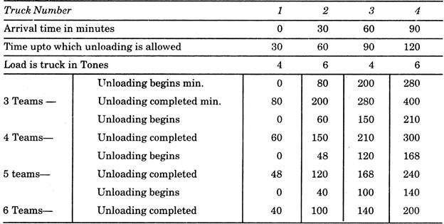
In this case, the time of arrival of first truck is assumed to be at zeroth minute. Hence the subsequent trucks will reach at 30th, 60th and 90th minutes. Now we calculate the unloading time by considering 3, 4, 5, and 6 teams for all the trucks.
Unloading time required for I truck of 4 tons by 3 teams @ 1 ton per hour per team
= 4/1 × 60/3 = 80 minutes
Therefore, unloading for II truck shall start after these 80 minutes and shall take unloading time of (for a load of 6 tons).
= 6/1 × 60/3 = 120 minutes
Hence unloading of II truck shall be completed at (80 + 120) = 200 minutes.
These calculations are now computed in the form of table shown below for unloading these 4 trucks, with the help of 3, 4, 5, or 6 teams:
The table shows that (e.g. for 3 teams) first truck was being unloaded for 80 minutes means it was detained for 50 min. extra. Second truck which arrived at 30th minute and should have been freed at 60th min. is required to wait for 140 min. extra, similarly III truck and IV truck was required to wait for 190 min, and 280 min. extra respectively.
Similarly waiting time is calculated when 4, 5 or 6 teams were employed for unloading, as shown in the table below:
Calculation of Detention Time of Trucks in Minutes:
Now we analyse the cost: Cost Analysis:
This shows that 5 teams give minimum cost. Table shows that total cost decreases when number of teams increase till it reaches to 5 teams, thereafter cost again increases when more number of teams are engaged.
Therefore, we should employ 5 teams, i.e., 10 workers to get optimum results.
Method # 6. Dynamic Programming:
Dynamic programming is a mathematical technique for solving problems where a sequence of decisions are involved. In such problems, there are number of stages and at each stage there are several alternatives available.
The decisions taken at stage one, act as conditions of the problem for stage two and so on, i.e. the decision taken at stage one affects the choice of decision at the stage two and so on. The basis of this is to select the best amongst the final possible alternative decisions, ignoring all other alternatives, which do not lead to the best (i.e. optimum).
Dynamic programming thus attempt to break large, complex problems into a series of smaller problems that are easier to solve separately. In this way, dynamic programming divides the problem into a number of sub-problems or decision stages. This technique is advantageous for solving problems, even when incorrect or less-than optimal decisions might have been taken in the past, and enables manager to make decision for future periods.
Dynamic programming is used in production scheduling, maintenance and repair, financial balancing, inventory, equipment replacement etc.
This can be better understood by following example:
Example 11:
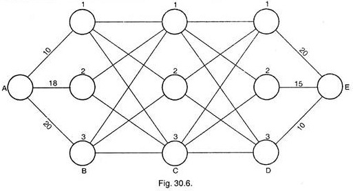
A pipe line is to be laid between stations A and E passing successively through one node of each B, C and D as shown in the figure below. The costs for lying from A and B and from D to E are shown in the figure while the costs between B and C and between C and D are given in the table below. We are required to find out the path which will require minimum costs of laying the pipe line from A to E.
Costs from B to C and C to D:
Solution:
Stage I:
In such problems, solution begins from the destination E and proceeds backwards, and in first stage determine minimum cost path between D1E, D2E and D3E. In this example, since there is only one path from each node on D to E, hence all these paths are optimum.
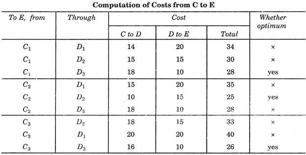
Costs from C to E:
Stage II:
Now we shift C to D, and observe that many more possibilities open. For example, from C1, path may pass from D1, D2 and D3 on its way to E.
The cost of each of these paths is calculated and the optimum is noted as shown in the table below:
This shows that, in passing from C1E, the path of minimum cost is through D3 and similarly minimum cost path from C2E and C3E is through D2 and D3 respectively. From this point, we start taking benefit of dynamic programming. From here, whenever path from C1 is required, we may follow it through D3. (Since we now know that optimum path from C1 to E is through D3).
Stage III:
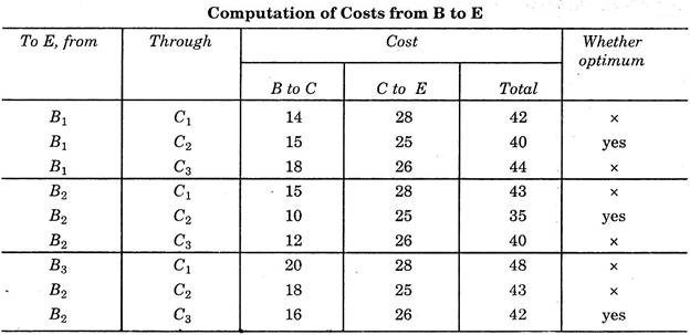
In the next stage, we further proceed backwards to point B, and starts examining the optimum costs from various nodes of point B, as shown in the table. In this table, instead of taking all the paths, we take use of optimum paths calculated above from C1, C2 and C3.
This shows that out of 3 possibilities from B1 to E, the path pass through C2 is optimum and similarly optimum cost path for B3E and B2E are through C2 and C3 respectively.
Stage IV:
Now in the last stage, we start from point A and compute the cost for the three possibilities below:
This shows that minimum cost from A to if is 50. And the optimum cost paths is A – B1 – C2 – D2 – E.
In this problem, total numbers of possible paths are 3 × 3 × 3 × 3 = 81. But by adopting dynamic programming, we have to make only 24 calculations. This shows that through this method, lot of labour could be saved.
