In this article we will discuss about the Markowitz mean-variance analysis and its importance in portfolio management.
Mean-Variance Theory:
Concept of Mean Variance:
Harry Markowitz is regarded as the father of modern portfolio theory. According to him, investors are mainly concerned with two properties of an asset: risk and return, but by diversification of portfolio it is possible to tradeoff between them. The essence of his theory is that risk of an individual asset hardly matters to an investor. What really counts is the contribution it makes to the investor’s total risk.
By turning his principle into a useful technique for selecting the right portfolio from a range of different assets, he developed ‘Mean Variance Analysis’ in 1952. The thrust has been on balancing safety, liquidity and return depending on the taste of different investors.
The portfolio selection problem can be divided into two stages, first finding the mean-variance efficient portfolios and secondly selecting one such portfolio. Investors do not like risk and the greater the riskiness of returns on an investment, the greater will be the returns expected by investors.
There is a trade-off between risk and return which must be reflected in the required rates of return on investment opportunities. The standard deviation (or variance) of return measures the total risk of an investment. It is not necessary for an investor to accept the total risk of an individual security. Investors can and do diversify to reduce risk. As number of holdings approach larger, a good deal of total risk is removed by diversification.
Assumptions:
It is a common phenomenon that the diversification of investments in the portfolio lead to reduction in variance of the return, even for the same level of expected return. This model has taken into account of risks associated with investments – using variance or standard deviation of the return.
This model is based on the following assumptions:
1. The return on an investment adequately summarizes the outcome of the investment.
2. The investors can visualize a probability distribution of rates of return.
3. The investors’ risk estimates are proportional to the variance of return they perceive for a security or portfolio.
4. Investors base their investment decisions on two criteria i.e., expected return and variance of return.
5. All investors are risk averse. For a given expected return he prefers to take minimum risk, obviously for a given level of risk the investor prefers to get maximum expected return.
6. Investors are assumed to be rational in so far as they would prefer greater returns to lesser ones given equal or smaller risk and risk averse. Risk aversion in this context means merely that, as between two investments with equal expected returns, the investment with the smaller risk would be preferred.
7. ‘Return’ could be any suitable measure of monetary inflows such as NPV, but yield has been the most commonly used measure of return, in this context, so that where the standard deviation of returns is referred to we shall mean the standard deviation of yield about its expected value.
Efficient Frontier:
Markowitz has formulized the risk return relationship and developed the concept of efficient frontier. For selection of a portfolio, comparison between a combination of portfolios is essential.
As a rule, a portfolio is not efficient if there is another portfolio with:
1. A higher expected value of return and a lower standard deviation (risk),
2. A higher expected value of return and the same standard deviation (risk),
3. The same expected value but a lower standard deviation (risk).
Markowitz has defined the diversification as the process of combining assets that are less than perfectly positively correlated in order to reduce portfolio risk without sacrificing any portfolio returns.
If an investor’s portfolio is not efficient he may:
a. Increase the expected value of return without increasing the risk,
b. Decrease the risk without decreasing the expected value of return, or
c. Obtain some combination of increase of expected return and decreased risk.
This is possible by switching to a portfolio on the efficient frontier.
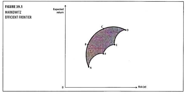
If all the investments are plotted on the risk-return sphere, individual securities would be dominated by portfolios, and the efficient frontier would be taken shape indicating investments which yield maximum return given the level of risk bearable, or which minimizes risk given the expected level of return. Figure 39.1 depicts the boundary of possible investments in securities A, B, C, D, E and F; and B, C, D are lying on the efficient frontier.
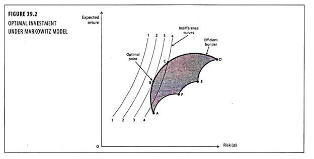
The best combination of expected value of return and risk (standard deviation) depends upon the investors utility function. The individual investor will want to hold that portfolio of securities that places him on the highest indifference curves, choosing from the set of available portfolios.
The dark line at the top of the set is the line of efficient combinations, or the efficient frontier. It depicts the trade-off between risk and expected value of return. The optimal investment achieved at a point where the indifference curve is at a tangent to the efficient frontier. This point reflects the risk level acceptable to the investor in order to achieve a desired return and provide maximum return for the bearable level of risk.
The concept of efficient frontier, and the optimal point location is explained with help of figure 39.2.
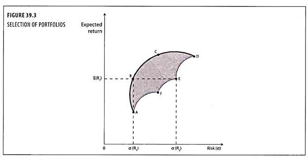
Figure 39.3 shows that A, B, C, D, E and F define the boundary of all possible investments out of which investments in B, C and D are the efficient proposals lying on the efficient frontier. The attractiveness of the investment proposals lying on the efficient frontier, depends on the investors attitude to risk. At point B, the level of risk and return is at optimum level. The returns are highest at point D, but simultaneously it carries higher risk than any other investment.
The shaded area represents all attainable portfolios and all the combinations of risk and expected return which may be achieved with the available securities. The efficient frontier denotes all possible efficient portfolios and any point on the frontier dominates any point to the right of it. For example, consider the portfolios represented by points B and E portfolios.
B and E promise the same expected return E(R1) but the risk associated with B is σ (R1) whereas that associated with E is σ (R2). Investors, therefore, prefer portfolios on the efficient frontier rather than interior portfolios given the assumption of risk aversion, obviously, point A on the frontier represents the portfolio with the least possible risk, whilst D represents the portfolio with the highest possible rate of return with highest risk.
The investor has to select a portfolio from amongst all those represented by the efficient frontier. This will depend upon his risk-return preference. As different investors have different preferences with respect to expected return and risk, the optimal portfolio of securities will vary considerably among investors.
Capital Market Line (CML):
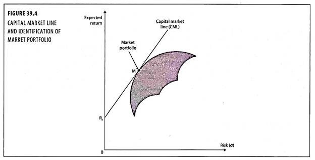
The Markowitz mean-variance analysis is modified by introducing into the analysis the concept of risk-free asset. If it is assumed that the investor has access to risk-free securities (for example, treasury bills) in addition to the universe of risky securities, then he can construct a new set of portfolios as depicted by the line RfM. At point Rf the investor is investing all his investible fund in risk-free securities, whilst at point M he is holding an all-equity portfolio.
The combination of risk-free investment and risky investments in portfolio which may be achieved by points between these two limits are termed ‘lending’ portfolios. Let us now assume that the investor can lend and borrow funds at the same risk-free interest rate. In such circumstances the efficiency boundary simply becomes the straight line drawn from Rf which is a tangent to the original risky portfolio efficiency boundary.
The efficiency boundary that arises out of this assumption of the identical risk free lending and borrowing rates leads to some very important conclusions and is termed as ‘capital market line’ (CML). The CML represents the tradeoff between risk and return available in the capital market.
Because the CML slopes upward, it reveals graphically that the acquisition of greater expected return requires that the investor accept more risk.
The slope of the CML is the rate of exchange between expected return and risk, and is given by:
The slope of the CML gives the market price of risk for fully diversified portfolios. The CML pertains only to well diversified portfolios. The CML, by using standard deviation as its risk measure, shows graphically the total risk of the individual securities and portfolios in the risk – return space. Individual securities do not lie on the CML because they bear same non-systematic risk, and non-systematic risk does not contribute to expected return.
CML and SML: Distinction:
CML stands for ‘Capital Market Line’ and SML stands for ‘Security Market Line’.
The difference between CML and SML are as follows:
1. While standard deviation is the measure of risk in CML, beta coefficient determines the risk factors of the SML.
2. The CML is a line that is used to show the rates of return, which depends on risk-free rates of return and levels of risk for a specific portfolio. SML which is also called a ‘Characteristic Line’, is a graphical representation of the market’s risk and return at a given time.
3. While the CML graphs define efficient portfolios, the SML graphs define both efficient and non-efficient portfolios.
4. The CML is considered to be superior when measuring the risk factors.
5. Where the market portfolio and risk free assets are determined by the CML, all security factors are determined by the SML.
Separation Theorem:
Investors can lend and borrow unlimited amounts at the risk-free interest rate of Rf, is important because of the fact that in such circumstances all risk averse investors will be interested in only one portfolio of risky investments i.e. Portfolio M as shown in figure 39.4.
They will either put all their investment funds into this portfolio or only part of their funds and lend the rest at the risk-free interest rate, or borrow additional funds and place all their own funds plus the borrowed funds into portfolio M.
Therefore, whatever investment portfolio is constructed by an investor, he will only be interested in one portfolio of purely risky assets. This will be portfolio M. As a result we are now in a position of being able to identify the portfolio of risky assets that an investor would wish to hold (i.e. ‘M’), without any knowledge of his set of indifference curves (except to assume that he is generally risk averse). This is called ‘separation theorem’.
Market Portfolio:
If all investors display the characteristics in separation theorem as described earlier, then portfolio M of the investors must consist of shares in all the companies quoted on the stock exchange. Hence it is termed as the ‘market portfolio’. An investor who wishes to hold the market portfolio as part of his overall investment portfolio would (at least in theory) hold shares in all the companies quoted on the stock market, in amounts proportionate to their total market values.
The concept of the market portfolio produces a definition of equilibrium market prices. If the market portfolio contains the shares of all the quoted companies, then the market prices of those shares (and hence the return they are expected to produce) must be such that they are acceptable investments for inclusion in the market portfolio. In other words, share prices are at equilibrium when they produce an expected return that is just sufficient compensation for the risk that they involve.


