After reading this article you will learn about:- 1. Introduction to O.C. Curves 2. O.C. Curves for Single Sampling Plan 3. O.C. Curves for Double Sampling Plan 4. Zones.
Introduction to O.C. Curves:
O.C. curves quantifies manufacturer’s (producer’s) risk and consumer’s (purchaser’s) risk. This is a graph of the percentage defective in a lot versus the probability that the sampling plan will accept a lot.
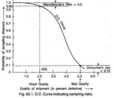
An O.C. Curve drawn for sampling plan of n = 300 and C = 10 at Fig. 60.1 indicates the following:
AQL = 0.02 or 2%
Manufacturer’s risk = 0.05
Consumer’s risk = 0.10
LTPD = 0.05 or more defectives.
All practical sampling plans have an operating characteristics curve, briefly called O.C. curve.
Following points need emphasis regarding O.C. curves:
(i) There is some chance that good lots will be rejected.
(ii) There is some chance that bad lots will be rejected.
(iii) These risks can be calculated by the theory of probability and depends on the number of samples inspected, the acceptance number, and the percent defectives in the lot offered for sample inspection. Given the amount of risks which can be tolerated, a sampling plan can be devised to meet these requirements.
(iv) The larger the sample used for inspection, the nearer the O.C. curve approaches the ideal. However beyond a certain point, the added cost in inspecting a large number of parts far exceeds the benefit derived.
In any acceptance sampling plan, three parameters are specified. The first parameter is number of articles N in the lot from which sample is to be drawn. The second parameter is the number of articles n in the random sample drawn from the lot, and the third is the acceptance number C.
This acceptance number C is the maximum allowable number of defective articles in the sample. If more than C defectives are found in a sample the lot is liable to be rejected. Since the lot size has little affect on the probability of acceptance, therefore lot size is generally ignored in deriving a sampling plan.
O.C. curve of an acceptance sampling plan (i.e. for a particular combination of n and C) shows how well the sampling plan discriminates between good and bad lots. In order to examine the suitability of an acceptance sampling plan, it is necessary to compare their performance over a range of possible quality levels of the product.
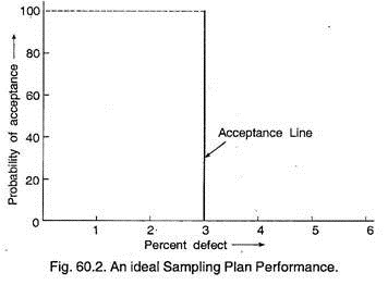
The graph of this performance is known as operating characteristic curve. Fig. 60.2 below shows an ideal O.C. curve where it is desired to accept all lots having 3% or less defectives, and to reject all lots having more than 3% defectives.
In this curve, all lots with less than 3% defectives have a probability of acceptance of 100%, while all lots with more than 3% defectives have a probability of acceptance as 0%. However such a plan does not exist in reality.
O.C. Curves for Single Sampling Plan:
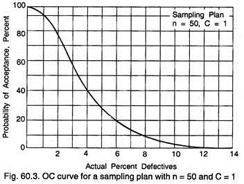
Graph 60.3 is an OC curve for a sampling plan with n = 50 and C = 1.
Graph shows the probability of acceptance of lot for various values of percent defectives in the lot. Suppose, if the actual bad quality were 1 percent, samples of n = 50 would accept the lot as satisfactory about 94 percent of the time and reject it about 6 percent of the time.
Note however that if the actual quality of the lot were somewhat worse than 1% defective, say 5% the probability of accepting these lots drastically to about 29%. This is the situation, we would like in a sampling plan. If the actual quality is good, then there should be a high probability of acceptance, but if the actual quality is poor, then the probability of acceptance should be low. Thus in this way the OC curve shows how well a given sampling plan discriminates.
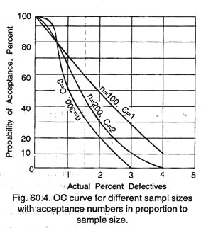
The discriminating power of any sampling plan depends largely on the size of the sample. Graph 60.4 shows the OC curves for sample sizes of 100, 200 and 300 with the acceptance number remaining in the proportion to the sample size. Graph 60.4 shows that the OC curve becomes steeper as the sample size goes up.
If the discrimination power of all the three plans shown in the graph is compared, it is found that these would accept lots of about 0.7% defectives about 80% of the time (the approximate cross over points of the three curves).
However, if actual quality fall to 3 percent defectives, the plan with n = 100 accepts lots about 25% of the time, n = 200 about 10% of the time, and n = 300 less than 1% of the time. Therefore, it shows that the plans with larger sample sizes are definitely more effective.
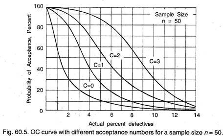
What happens to the OC curve, if any of the acceptance number changes? Graph 60.5 shows OC curves for sample of n = 50 and acceptance number of C = 0, 1, 2 and 3. Graph indicates that the effect is mainly to change the level of the OC curve so that lower acceptance number makes the plan “tighter”.
A sampling plan that discriminated perfectly between good and bad lots would have an OC curve that was vertical; that is, it would follow the dashed lines of Graph 60.4. For all lots having percent defectives to the left of the dashed line, the probability of acceptance is 100.
For all lots having percent defectives to the right of the line the probability of acceptances is zero but the only plan which could achieve this discrimination is one requiring cent percent inspection. Therefore, the proper justification for the selection of a sampling plan is the balance between inspection costs and the probable cost of rejected parts.
By making sampling plans more discriminating (increasing sample size) or tighter (decreasing acceptance numbers), we can approach any desired level of outgoing quality that we please but at increasing inspection cost. This increased inspection effort would result in lower probable costs of passing defectives and at some point the combination of the incremental costs is a minimum.
This minimum point defines the most economical sampling plan for a given situation.
O.C. Curves for Double Sampling Plan:
Double sampling plans are generally specified by following:
n1 = number of items in the first sample,
c1 = acceptance number for the first sample (i.e. maximum number of defectives that will permit the acceptance of the lot on the basis of first sample)
n2 = number of items in the second lot
c2 = acceptance number for the two samples combined (i.e. maximum number of defectives that will permit the acceptance of the lot on the basis of two samples.
For example, interpretation of following sampling plan is given hereunder:
n1 = 30, c1 = 0, n2 = 60, c2 = 3
1. Inspect a first sample of thirty items from a lot.
2. Accept the lot on the basis of first sample, if the sample contains O defectives.
3. Reject the lot on the basis of first sample, if the sample contains more them 3 defectives.
4. Inspect a second sample of 60 items, if the first sample contains 1, 2 or 3 defectives.
5. Accept the lot on the basis of both the samples combined together (30 + 60 = 90 items), if the defectives are 3 or less.
6. Reject the entire lot on the basis of combined sample, if the defectives are more than 3 items.
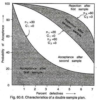
Fig. 60.6 shows three O.C. curves involved in the analysis of this double sampling plan.
These three curves divide the figure in four zones indicating following possibilities for acceptance or rejection:
1. I zone (lowest zone)/Acceptance after first sample.
2. II zone (highest zone)/Rejection after the first sample.
3. III zone (lower without hatching zone)—Acceptance after second sample.
4. IV zone (higher with hatching zone)—Rejection after second sample.
Characteristics of the lowest curve is n = 30 and C = 0.
Characteristics of the highest curve is n = 60 and C = 3.
Characteristics of the middle curve is the actual O.C. curve of the double sampling plan.
Zones of O.C. Curve:
O.C. curve can be divided into following 3 zones:
(a) Acceptance Zone:
In this zone all the batches are accepted, therefore, the O.C. curve should be so selected that its acceptance zone accepts what is considered to be satisfactory lot.
(b) Rejection Zone:
In this zone, all the batches are rejected. Hence the O.C. curve selected should be such that it rejects what is considered to be an unsatisfactory lot.
(c) Zone of Indecision:
This is the zone where there is no purity that whether any particular batch or lot will be accepted or rejected. This problem can be solved either by adopting 100% inspection or by taking larger sample, but these will increase the inspection costs.
A batch or lot in this zone is worse than acceptable lot, and better than those what is considered as unacceptable. Thus its quality is border-line, and practically does not matter much whether a lot is finally accepted or rejected from this zone.
