In this article we will discuss about the formulation of Linear Programming Problem (LPP). Also learn about the methods to find optimal solution of Linear Programming Problem (LPP).
Formulation of Linear Programming Problem (LPP):
The construction of objective function as well as the constraints is known as formulation of LPP.
The following are the basic steps in formulation of LPP:
(i) Identify the variables to be determined and then express these by some algebraic symbols.
ADVERTISEMENTS:
(ii) Locate the various constraints/restrictions present in the problem and express these as linear equations/inequalities which are some linear functions of the variables identified in step (i).
(iii) Determine the objective of the problem and express it as linear function of the decision variables involved in the phenomenon.
The technique is illustrated by the following example:
Example 1:
ADVERTISEMENTS:
An electronic firm is undecided at the most profitable mix for its products. The products manufactured are transistors, resistors and carbon tubes with a profit of (per 100 units) Rs. 10, Rs. 6 and Rs. 4 respectively. To produce a shipment of transistors containing 100 units requires 1 hour of engineering, 10 hours of direct labour, and 2 hours of administrative service. To produce 100 units of resistors requires 1 hour, 4 hours and 2 hours of engineering, direct labour and administrative times respectively. For 100 units of carbon tubes it needs 1 hour, 6 hours and 5 hours of engineering direct labour and administrative times respectively.
There are 100 hours of engineering time, 600 hours of direct labour and 300 hours of administrative time available. Formulate the corresponding LPP.
Solution:
Let the firm produce X hundred units of transistors, Y hundred units of resistors and Z hundred units of carbon tubes. Then the total profit to be maximized from this output will be
ADVERTISEMENTS:
P = 10X + 6Y + 4Z
This is our objective function.
Now production of X hundred units of transistors, Y hundred units of resistors and Z hundred units of carbon tubes will require X + Y + Z hours of engineering time, 10X + 4Y + 6Z hours of direct labour time and 2X + 2Y + 5Z hours of administrative service.
But the total time available for engineering, direct labour and administrative services is 100,600 and 300 hours respectively.
ADVERTISEMENTS:
Hence the constraints are:
X + Y + Z ≤ 100
10X + 4Y+ 6Z ≤ 600
2X + 2Y + 5Z ≤ 300
ADVERTISEMENTS:
with X, Y, Z ≥ 0 as the non-negativity restriction.
Thus the formulated l.p.p. is Maximise
M = 10X + 6Y + 4Z
s.t. X + Y + Z ≤ 100
ADVERTISEMENTS:
10X + 4Y + 6Z ≤ 600
2X + 2Y + 5Z ≤ 300
X, Y, Z ≥ 0.
It is evident that the word linear programming implies that all the constraints and the objective function are expressed as linear functions of the variables. Linear relationship means that when one factor changes so does another by a constant amount.
Solution of Linear Programming Problems:
There are many methods to find the optimal solution of l.p.p.
ADVERTISEMENTS:
The methods are:
(i) Graphical Method.
(ii) Simplex Method.
(iii) Degeneracy Method.
(i) Graphical Method:
The industrial problems involving two or three variables can be easily and effectively solved by drawing the graph for various constraints and the objective function. It is even simpler for two variable cases as three-dimensional geometry is rather difficult to draw on graph paper.
ADVERTISEMENTS:
The following are the steps in Graphical Solution of l.p.p:
(i) The constraints of the problem are taken as equalities and plotted on the graph paper. The region satisfying each constraint is determined and then the region common to all the constraint relations is located. This region is known as feasible region for the problem as all points lying in this region will simultaneously satisfy the given constraints.
The solution set of the system of constraints is found to be represented by some convex polygon termed as feasible region.
(ii) Objective function is also plotted on the same graph paper by taking some arbitrary value of Z.
(iii) Trial and error method is used to locate the optimal solution inside the feasible region determined in step (i) so that the objective function is optimized. It is experienced that the optimal solution is located near the extreme points of the feasible region. Thus the optimum feasible point should be searched only at the corners of the convex polygon.
The graph for all the constraints and the objective function will be straight lines in I.pp.
ADVERTISEMENTS:
The method is illustrated with following examples:
Example 2:
A resourceful home decorator manufactures two types of lamps A and B. Both the lamps go through two technicians first a cutter and then a finisher. Lamp a requires one hour of cutter time time and two hours of finisher’s time. The cutter has 104 hours and finisher 76 hours of finisher’s time. Profit on one lamp of A is Rs. 6.00 and one lamp of B is Rs. 11.00. Assuming that the decorator can sell all that he produces, how many of each type of lamps should he manufacture to obtain the best return? Find the optimum solution by graphical method.
Solution:
Here the objective function and the constraints are
Max. Z = 6X + 11Y
ADVERTISEMENTS:
2X + Y ≤ 104
X + 2Y ≤ 76
X, Y ≥ 0
In a two dimensional space, the non-negativity restriction will be satisfied in 1st quadrant only. Thus the first quadrant will be the perspective feasible region.
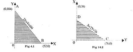
Again the constraints are linear functions of X and Y. So to plot each line on the graph paper we require at least two points e.g. for the constraints 2X + Y ≤ 104, we first convert it into equality by writing 2X + Y = 104 and then find the co-ordinates lying on the line by first putting X = 0 and finding corresponding value of Y and then putting Y = 0 in the equation and finding the corresponding value of X i.e.. Y for X = 0, we get 2(0) + Y = 104, i.e. Y = 104 and for Y = 0, we get 2X + Y – 104 i.e., X = 52. Hence the two points lying on the line 2X + Y = 104 are A = (0, 104) and B = (52, 0).
Fig.14.1 shows the area containing all those values of X and Y for which the constraint 2X + Y ≤ 104 will be satisfied. The diagonally sloping line AB is the constraint. Now for second constraint X + 2Y ≤ 76 the two points corresponding to line X + Y = 76 can be calculated as C = (76, 0) and D = (0, 88) and the feasible area on the graph is shown in Fig.14.2. The feasible region in this case is area OCD.
The objective function can be plotted by taking some arbitrary value of Z. Taking Z = 66, we get
6X + 11Y = 66
and the two points corresponding to this line area given as (0,6) and (11,0).
Fig. 14.3 corresponds to the objective function for some arbitrary value of Z. Iso-contribution lines for different values of Z can be drawn by drawing the lines parallel to the line P1 P1 , i.e. P2, P2, P3 P3 and so on. The lines closer to the origin produce less total contribution and the lines which farther out produce more contribution.
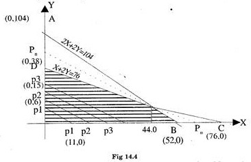
To maximise the objective function we should move to the farthest point till the iso-contribution line touch one point in the feasibility area. For this the fig. 14.1, 14.2 and 14.3 are drawn on one graph in fig. 14.4.
In Fig 14.4 the region ODQB in common to the feasible regions of inequalities
ADVERTISEMENTS:
2X + Y ≤ 104 and X + 2Y ≤ 76
Hence all point lying in this region will satisfy both the constraints of the problem. Thus ODBQ is our required feasible region.
Now the iso-contribution line p1 p1 is moved to-wards right by drawing lines parallel to it till it touches the farthest point of the feasible region ODQB, which evidently is the point Q. The co-ordinates for point Q are (44,15). Thus the maximum profit is given by
Z = 6(44) + 11(15)
= 264 + 165 = Rs.429
and X = 44 and Y = 15 is the optimum solution of the problem.
(ii) Simplex Method:
Simplex method is the most general and powerful technique to solve l.p.p. It is an iterative procedure, which either solves l.p.p. in a finite number of steps or gives an indication that there is an unbounded solution to l.p.p. Simplex method is designed to solve simultaneously a system of linear equations where there are more/less unknowns than the number of equations.
To solve a problem by simplex method requires:
(i) Arranging the objective function and constraints in a special way and
(ii) Following a systematic procedure and a set of rules in finding the desired solution.
The first step in all types of l.p.p. solved by simplex method is to formulate the problem in the form of objective function and the constraints. Essentially the simplex method searches through combinations of solutions until the best solution is found.
Introduction of Slack, Surplus and Artificial Variables in l.p.p:
The inequalities having ≤ or ≥ signs are converted into equalities using slack and artificial variables.
The following is the use and description of these variables:
(a) Slack Variables:
These variables are included in ≤ inequalities to convert them into equality e.g. given
a1 X + a2 Y ≤ b1.
We redefine it as a1 X + a2 Y + S1 = b1
where S1 is the slack variable.
i.e., Slack variable = Total Resource – Used resource
Slack variables are non-negative and explain the unallocated portion of the given limited resources. These permit more comprehensive economic interpretation of the solution.
(b) Surplus Variables:
These variables are introduced in ≥ in-equations to change them into equations e.g.
a3 X + a4 Y ≥ b2
is written as a3 X + a4 Y – S2 = b2.
where S2 is surplus variable. Here
Surplus = Production – Requirement.
The value of this variable can be interpreted as the amount over and above the required minimum level. It is also non-negative.
(c) Introduction of Artificial Variables in Optimization Problems:
In many cases the constraints are a combination of ≥, ≤ and = in-equations and equations. It is observed that the introduction of surplus variable is not able to provide the initial feasible solution. To solve the problem artificial variables are introduced. The artificial variables are fictitious and cannot have any physical meaning.
A very large penalty denoted by M per unit is assigned in objective function to the artificial variables designated as -M in the case of maximization problems and +M in the case of minimisation problems. The high value of M renders inclusion of artificial variables in the solution prohibitively costly e.g. given the constraints
C1 X1 + C2 X2 ≤ a1
C3 X1 + C4 X2 ≥ a2
Cs X1 + C6X2 = a3
the ≤ and ≥ in equations are changed into equations by adding slack and surplus variables i.e. taking
C1X1 + C2 X2 + S1 = a1S1 is slack variable.
C3X1 + C4X2 – S2 = a2, S2 is surplus variable.
The need for artificial variable in ≥ in equation arises, as the surplus variable S2 does not satisfy the non-negativity condition of basic feasible solution.
The reason being that none of the basic variables in our problem can have a negative value. It is observed that introduction of surplus variables with a negative sign in ≥ inequalities does not provide the initial feasible solution, as it cannot be one of the variables. In the initial feasible solution. Thus the artificial variable A is included in the second constraint to write it as
C3X1 + C4X2 – S2 + A1 = a2
Also an artificial variable is included in the equation with equal to sign so that the equation has a basic variable.
C5 X1 + C6 X2 + A2 = a3
Note:
A variable is said to be a basic variable in an equation if it appears with a unit co-efficient in that equation and zero co-efficient in all other equations.
The variables taken in the initial feasible solution are chosen corresponding to identity vector columns i.e. of the form (1, 0, 0), (0, 1, 0), (0, 0, 1) initial simplex tableau giving priority to artificial variables. The artificial variables are to be first removed from the solution basis.
For this, if at any iterative stage of simplex method, the basic feasible solution contains artificial variables but the variable to be deleted at that stage is not an artificial variable then one can depart from the simplex criterion for selecting the entering variable.
In simplex method all variables must appear in all the equations. This is done by adding the variables absent in an equation with zero coefficients. All variables should also appear in objective function with zero profit or cost for surplus and slack variables and very high penalty M for artificial variables. M is included with a negative sign in maximization problems and with a positive sign in minimisation problems.
Simplex Procedure:
The first step in simplex procedure is to introduce slack, surplus and artificial variables in in-equations to change them into equations and also in the objective function.
After this the objective function and the constraints are arranged in a special way i.e. all variables, real, surplus, slack and artificial are arranged in the same order in all constraints and the objective function. Thus the constraints equations are expressed is a canonical system from which a basic feasible solution can be easily obtained. This is known as standard form of l.p.p.
The next step is to prepare the initial simplex tableau.
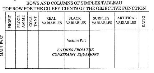
The following are the main columns of a Simplex Tableau:
The number of rows in main part of the simplex tableau is equal to the number of constraints in the system. The number of column in the variable part of the table depends on the number of slack, surplus, artificial and real variables in the system under study. The remaining column and rows of the simplex tableau are calculated step by step.
The construction of the initial simplex tableau is explained with the help of l.p.p. formulated in Examples 2.
Here we have:
Z = 6X + 11Y
2X + Y ≤ 104
X + Y ≤ 76
X, Y ≥ 0
Adding slack variables in constraints and objective function, and arranging it in standard from, we get:
Z = 6X + 11Y + 0.S1 + 0.S2
2X + Y+ S1 + 0.S2 = 104 ….I
X + 2Y+ 0.S1 + S2 =76 ….II
Now the initial Simplex Tableau column will be
Key Column:
The entries of the initial simplex Tableau can be made in the following manner:
(i) Top-Row:
This row begins above the constant column and ends above the column corresponding to the last variable appearing in the problem. The column corresponding to the last variable appearing in the problem.
The column corresponding to constant column in this row is allocated the word C The other columns of this row are assigned the coefficients of the corresponding variables in the objective function, viz. columns corresponding to real variables contains the co-efficient of the corresponding real variables in the objective function and the column above the slack variable column constraints the co-efficient of the corresponding real variables in the objective function and the columns above the slack variable columns contains the co-efficient of the corresponding slack variables in the objective function.
Thus the top row is:
ROW.I. entries from constant column to the last variable column are respectively, the constant value on right hand side and the coefficients of real and slack variables in equation I i.e.
Similarly the entries of ROW II corresponds to the equation II of the problem i.e.
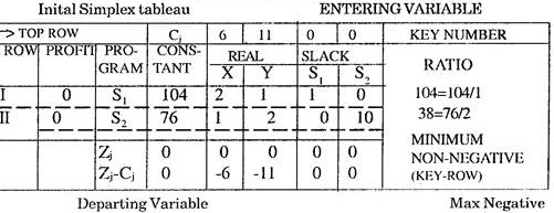
At the stage, top row and ROW I and ROW II of the initial simplex table can be written as,
The entries in profit and programme column of initial simplex tableau are made by locating the basic solution variables from the initial simplex tableau.
The basic solution variables can be located by following steps:
(i) Locate the unit/Identity column vectors among the variable columns of the initial simplex tableau. These are the columns which contain one element as (+1) and all other elements zero e.g. in the above table the columns for S1 and S2 are unit vectors with values (1, 0) and (0, 1) respectively.
Now in column for S1, 1 appears in 1st row, so S1 is entered in program column of 1st row. Similarly S2 is entered in program column of 2nd row. These are the variables entering in the initial feasible solution. The variable S1 lies in Programme column of Row I and its coefficient in the objective function i.e. 0 is entered in Profit column of Row I. Similarly, corresponding to variable S2 of Programme Column in Row II, its coefficient 0 in objective function is entered in Profit column of Row II.
Upto this point the initial simplex tableau is prepared only with the help of the objective function and the constraint equations with no calculations.
Now we have to determine, whether any improvement in the solution at this stage can be made or not. Because at this stage the basic feasible solution is S1 = 104, S2 = 76 with corresponding profits equal to zero. To determine this, two more rows Zj and Zj – Cj are added in the Simplex Tableau.
The values of Zj in column for X, Y, S1, and S2 are the amounts by which profit would be reduced if one unit of any of the variables X, Y, S1, S2 were added to the mix.
The values of Zj corresponding to S1, S2, X and Y are calculated as:
Rule 1:
Rule 2:
Now Cj has been defined profit per unit. Thus Zj – Cj is the net profit, which will result from introducing one unit of the corresponding variable to the production schedule or solution. Zj – Cj is also known as unit improvement.
Maximisation Problem:
By examining Zj – Cj row, we can see the change in profit for each variable and if this is positive for all variables then this indicates that the solution obtained is optimum and no improvement is possible. In case one or more values of Zj – Cj are found to be negative, then the solution needs improvement.
Note:
Some people prefer to calculate Cj – Zj. In that case optimum solution is reached if all Cj – Zj are negative. One or more positive value of Cj – Zj indicate need for improvement in the solution.
Rule 3: Improving upon the Initial Solution:
Simplex method is an iterative procedure where each step brings closer to the optimum solution. It is done by removing. One variable at a time from the program column and replacing it with a new one. The process is repeated a number of times till no further improvement in the solution is possible i.e. all-Zj – Cj are positive.
The decision of continuing the iterative procedure is taken by examining Zj – Cj row. If one or more columns of Zj – Cj row are found to have negative values, then there is a need to improve the solution.
Rule 4: Rules for Choosing the Variable to Enter the Program Column:
Examine Zj – Cj values at each iteration and locate the numerically largest negative value, larger the number greater the improvement possible e.g. inspection of Zj – Cj. values in initial simplex tableau tells us that – 11 is numerically most negative value. Hence the column containing the value – 11 is designated as key column at this iteration and the corresponding variable of this column i.e. Y is the new entering variable in the basis i.e. the program column of next tableau.
Rule 5: Rules for Determining the Outgoing Variable form the Basis:
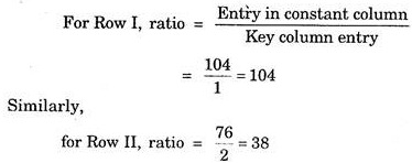
The next step is to determine which variable is to be replaced. For this ratio column is computed. This is done by dividing the entry in constant column of a row by the corresponding value in key column e.g. in our illustration.
Now we examine the ratio column of the simplex tableau and select the row with smallest non-negative ratio and call it key row. The variable lying in the program column of key row is the leaving variable at the iteration e.g. Row II is the key row and S2 variable of program column is replaced by the entering variable Y. The value lying at the intersection of key row and key column is known as Key Number.
Entering Variable:
Rule 6. Development of Second Simplex Solution:
The coefficient values in the body of each iteration tableau are really rates of substitution between all the variables.
In the new tableau the key row is replaced by the row obtained by dividing each entry of the key row by the key number. In our example the new row II will be:
Note that variable S2 is replaced by Y and in profit column we write the value of Cj row corresponding to key column i.e. value of Cj = 11
Rule 7: To Complete the Second Tableau, New Values for Remaining Rows are Computed by the Formula
[Elements in the old row] – [(element in the key column of that row) x (corresponding element in the row replacing key row)] = (new row)
e.g. in Row I of the initial simplex table the elements are (104, 2, 1, 1, 0).
So using the above formula, Row I in new tableau will be
(104,2, 1, 1, 0) – (1) (38 1/2 1 0 1/2)
= (104 – 38, 2 – .5, 1 – 1, 1 – 0, 0 – 0.5)
= (66, 1.5 0 1 – 1/2)
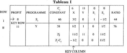
The new Simplex Tableau I is completed by entering the appropriate unit costs in profit column for the mix. variables e.g. In profit column of Tableau I, the per unit profit of Y i.e. 11 is entered. Thus the new Simplex Tableau I becomes.
Now Rules I, II, III, are again applied to know whether optimum solution stage has arrived or not. In Tableau I, Zj and Zj – Cj are calculated by the rules II and I. Now all Zj – Cj are not positive. Thus it is not the stage of optimum solution. There is one Zj – Cj corresponding to the column for variable X, which is negative. So by rule 4 this column is key column. Now applying rule 5 we calculate the Ratio column in tableau I and find the minimum positive value in ratio column.
The row containing this minimum positive value in ratio column is designated as key row at this stage. The variable appearing in the programme column of key row is departing variable. Thus Row I is the Key Row and X is the entering variable and S1 is the departing variable in the basis of Tableau I.
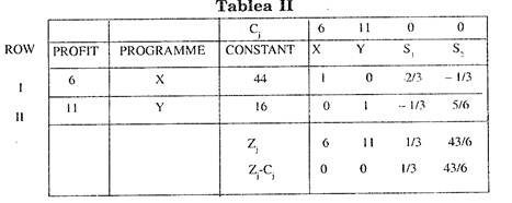
Now Tableau II is prepared from Tableau I using rules 6 and 7.
Row II in Tableau II is given by:
(38 0 1/2 1/2 1) – [(1/2) (44 2/3 – 1/3 1 0)] = (16 – 1/3 5/6 0 1)
Again Rules I, II and III are applied on Tableau II to find whether the solution is optimum or not. It is observed that in Tableau II all Zj -Cj are positive. Hence the optimum solution stage has been attained.
The optimum solution is X = 44, Y = 16 with a maximum profit of Rs. 440 which approximately is the same as in Example 2.
Steps in the Simplex procedure are listed below:
(i) Formulate the problem by determining the objective function and constraints.
(ii) Introduce slack, surplus and artificial variables in the objective function and the constraints by changing inequalities’ into equalities to get the standard form.
(iii) Prepare the initial Simplex tableau.
(iv) Apply rules I, II and III to determine whether the solution is optimum or not.
If the solution is not optimum, then go to steps 5 to 11.
(v) Determine the entering variable (key column) by selecting the column with most negative (Zj – Cj).
(vi) Determine the departing variable (key row) by calculating the Ratio column from Rule V and selecting the smallest non-negative value.
(vii) Compute the replacing row of the improved simplex tableau by rule VI.
(viii) Compute the remaining rows of the new table by rule VII.
(ix) Go to step (iv) and continue till optimum solution is obtained.
The application of simplex method is illustrated with the help of following example.
Example 3:
Two products A and B are processed on three machines M1 M2 and M3
The processing times per unit, Machine availability and profit per unit are given below:
Formulate the mathematical model and solve it by simplex method. Also find the number of hours machine M3 remains unutilized.
Solution:
Step 1:
Let X units of A and Y units of B be produced. Then the corresponding profit is 10X -12Y and the objective function is
Max. Z = 10X + 12Y
Now the constraints for the three machines will be:
2X + 3Y ≤ 1500 for M1
3X + 2Y ≤ 1500 for M2
X + Y ≤ 1000 for M3
X, Y ≥ 0 Non-negativity restriction.
Step 2:
Since all the constraints are having ≤ signs, slack variables can be introduced to change these in equalities. There are three constraints so three slack variables S1, S2 and S3 are introduced in the problem.
2X + 3Y + S1+ 0.S2+ 0.S3 = 15500
3X + 2Y + 0.S1 + S2 + 0.S3 = 1500
X + Y + 0.S1+ 0.S2+ S3 = 1000
and Max. Z = 10X + 12Y + 0.51 + 0.52 + 0.53
Step 3:
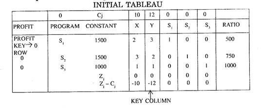
The initial simplex tableau can now be prepared
Program column entries are mad by locating unit column vectors corresponding to the variables S1, S2, S3. X and Y. Here these vectors are for variables S1 (1, 0, 0), S2 (0, 1, 0) and S3 (0, 0, 1). The initial feasible solution is given by the variables S1, S2 and S3 with total profit = 0.
Step 4:
Zj and Z j– Cj are calculated by Rules I, II and III. Now there are two negative values in Z j– Cj row of the initial simplex tableau. So the initial solution needs improvement.
Step 5:
From Rule IV the most negative value i.e. – 12 determines the key column and the real variable Y corresponding to this column is the entering variable.
Step 6:
Ratio column is calculated using Rule V and the least positive Ratio i.e. 500 in the Tableau determines the key row. Thus S1 is departing variable at this iteration.
Step 7:
Applying rule VI, we get the replacing row in Tableau I from key row in initial table. The row is
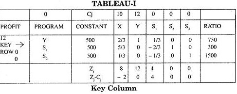
12 Y 500 2/3 1 1/3 0 0
Step 8:
The remaining rows of Tableau I are obtained by applying r Rule VII on the other rows of initial Simplex tableau and the replaced row in Tableau I. Thus the new Tableau I for the improved solution becomes.
Here Row = (1500 3, 2, 0 1 0) – 2 (500 2/3 1 1/3 0 0)
= (500 5/3 0 – 23 1 0)
Similarly Row III can be calculated.
Step 9:
It is observed from Zj – Cj row that Tableau I does not provide an optimum solution. Hence we again go to Step 4 to further improve the solution and get Tableau II.
In tableau II all Z j– Cj are positive. Hence the optimum solution is X = 300, Y = 300 and maximum value of Z = 6600.
The time utilised for machine M3 = 300 + 300 = 600 hours. Thus the unutilized time for machine M3 = 1000 – 600 = 400 hrs.
Minimisation Problem:
There may be situations where the objective may be to minimise the cost of production, duration of production etc. i.e. the objective function is to be minimised. In such cases the problem can be visualised as maximization problem by simply multiplying both the sides of the objective function by -1. Here minimisation of Z is equivalent to maximization of (- Z). The constraints remain unchanged.
The method is illustrated by the following example.
Example 4:
Z = 20 X1 + 10 X2
X1 + 2X2 ≥ 40
4X1 + 3X2 ≥ 60
3X1 + X2 ≥ 30
X1 .X2 ≥ 0
Solution:
The minimisation problem is changed into maximization problem, by taking
Max. Z* = – Z = – 20 X1 – 10 X2
Introducing slack, artificial and surplus variables in the problem, we get
X1 + 2X2 + S1 + 0.S2 + 0.S3 + 0.A1 + 0.A2 = 40
4X1 + 3X2 + 0.S2 + 0.S3 + A1 + 0.A2 = 60
3X1 + X2 + 0.S1 + 0.S2 – S3 + 0.A1 + A2 = 30
and Z* = – 20X1 – 10X2 + 0.S1 + 0.S2 + 0.S3 – MA1 – MA2
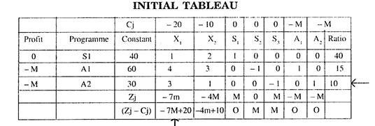
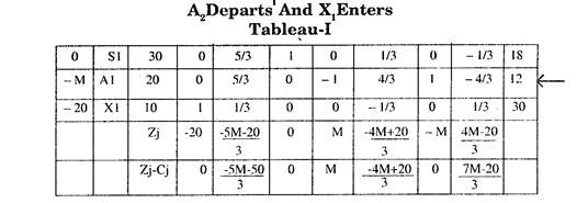
The various simplex tableau are now prepared to get the optimal solution.
Since M is quite large so M – 4 and M – 2 will be positive.
Thus in Tableau II all Zj– Cj are positive. Hence the optimum solution is X1, = 6, X2 = 12 and minimum value of Z = 240.
Problem of Degeneracy:
In many Linear Programming problems it is observed that at any iteration of the simplex method, two or more rows in Ratio column have identical least non-negative value. Then the question arises that which row should be taken as key row? This situation where at any iteration of simplex procedure two or more variables of the basis claim themselves to be departing variables is known as Degeneracy problem.
The problem of degeneracy can be experienced when one of the constraints have zero on its right hand side.
The problem of degeneracy can be resolved with following steps:
(i) Divide each element of the disputed rows (i.e. rows with identical non-negative minimum entry in ratio column of the simplex tableau) by the entry in the key column of the respective row.
(ii) The values obtained in step (i) are then compared step by step from left to right. Priority is given to identity columns for slack and artificial variables.
(iii) The search for key row terminates where the row yields unequal ratios. Row having algebraically smaller ratio is taken as the key row. The method is illustrated by the following example.
Example 5:
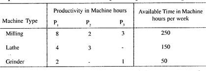
A manufacturing firm has discontinued production of a certain unprofitable product line. This created considerable excess production capacity. Management is considering to devote this excess capacity to one or more of the three products; call them P1, P2, and P3.
The available capacity on the machine as well as the number of machine hours required for each unit of the respective products is given below.
The unit profit would be Rs. 20, Rs. 6 and Rs. 8 respectively from P1, P2 and P3 Find how much of each product the firm should produce in order to maximise the profit?
Solution:
Let the firm should produce X units of P1, Y units of P2, and Z units of P3. Then the corresponding profit will be
Z = 20X + 6Y + 8Z
Thus the objective function is
Max. Z = 20X + 6Y + 8Z
Subject to the constraints
8X + 2Y + 3Z ≤ 250
4X + 3Y ≤ 150
2X + Z ≤ 50
X, Y, Z ≥ 0.
Introducing slack variables in the objective function and the constraints, the standard form becomes
Z = 20X + 6Y + 8Z + 0.S1 + 0.S2 + 0.S3
and 8X + 2Y + 3Z+ S1 + 0.S2 + 0.S3 = 250
4X + 3Y + 0.Z + 0.S1 + S2 + 0.S3 = 150
2X + 0.Y + Z + 0.S1 + 0.S2 + S3 = 50
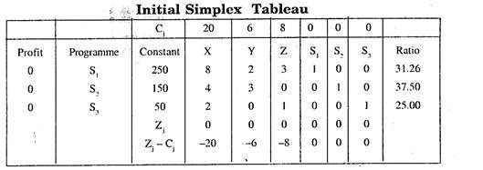
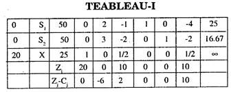
The various simplex tableau are now prepared to get the optimal solution.
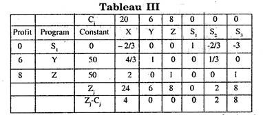
At this stage there are two non-negative minimum values in Ratio column of tableau II. Thus there is a problem of degeneracy. So we divide the I and the III rows by the elements of key column i.e. row I by 1/3 and row III by 1/2 and observe this ratio for S1, S2 and S3.
Comparing step by step from left to right, we observe that the ratio corresponding to column S1 in row III is least positive.
Hence at this stage Row III is taken as the key row and X becomes the departing variable whereas Z is the entering variable.
Note:
In case both the entries corresponding to column for S1, were identical then we should have moved to next column corresponding to S2.
Thus all Zj – Cj are positive. Hence the optimum solution is Y = 6, Z = 8, X = 0 and Max. Z = 700.
