Sales forecasting techniques may be categorized as follows:- 1. Historic Estimate 2. Sales Force Estimate 3. Trend Line (or Time Series Analysis) Technique 4. Market Survey 5. Delphi Method 6. Judgmental Techniques 7. Prior Knowledge 8. Forecasting by Past Average 9. Forecasting from Last Period’s Sales 10. Forecasting by Moving Average and Few Others.
Technique # 1. Historic Estimate:
This technique of sales forecasting makes use of the assumption that what happened in past will happen in future. For example if a concern has sold 5000 blankets in winter last year, it will be able to sell the same quantity in winter this year also. Historic estimate is useful if the activity is affected by pattern of seasonality.
It is useful for determining model, size and colour distribution. It is successful only when pattern of events remains unchanged, i.e., if economy is static. This is rarely true except for short periods of time. Historic estimate is not scientifically valid and thus it is not an accurate method; the total sales forecast provided by this method should be modified by other techniques.
Technique # 2. Sales Force Estimate:
This technique is based upon the principle-that the persons in contact with the market know best about the future market trends. Individual salesmen make sales estimates of their territories and submit it with the District Sales Manager who analyses it, modifies it and sends the same to Factory Sales Manager in consultation with other related factory executives formulates the final estimate of sales. This technique is useful when an industry is making a limited number of products (e.g., commercial power generating equipment) and there are a few large customers.
Technique # 3. Trend Line Technique:
ADVERTISEMENTS:
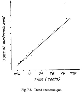
Trend line technique of sales forecasting is employed when there is an appreciable amount of historical data. This technique is more reliable than the historic estimate (a) above. This technique involves plotting historical data, i.e., a diagram (Fig. 7.3) between activity indicator, e.g., tons of material (say past sales) on y-axis and time on X-axis.
A single best fitting line (using statistical technique) is drawn and projected to show sales estimate for future. This technique is more accurate as it makes use of a large past data and possesses scientific validity. However, it is time-consuming, involves long mathematical calculations and assumes an infinite population of relatively small customers so that the decision of an individual customer cannot have an appreciable effect on total product demand.
Technique # 4. Market Survey, i.e. Market Research Technique:
This technique of sales forecasting finds application when a concern introduces a new product in the market and is interested to estimate its sales forecast. For a new product, naturally, no historic or past data regarding sales will be available. This technique may be very informal, utilizing the sales force to feel out the potential customers in order to establish the extent of the market or it may be a systematically conducted survey using special mathematical tools. Generally, the new product is introduced in a relatively small critical trial area, market reaction is noted and the total sales (country-wide) is projected from these results.
Technique # 5. Delphi Method:
ADVERTISEMENTS:
A panel of experts is interrogated by a sequence of questionnaires in which the response to one questionnaire is used to produce the next questionnaire. Any set of information available to some experts and not others is thus passed on to the others, enabling all the experts to have access to all the information for forecasting.
The method solicits and collates opinion from experts to arrive at a reliable consensus. This technique eliminates the bandwagon effect of majority opinion. Delphi method has fair to very good accuracy for short and long term forecasts. The method is applicable to forecasts of long-range and new-product sales.
Technique # 6. Judgmental Techniques:
They involve:
1. Opinions of Consumers and Customers:
ADVERTISEMENTS:
Questionnaires related to buying the product may be sent to a selected group of consumers and to the customers who have already purchased the product. The information thus received can be very useful in estimating product performance and its probable demand in future.
2. Retail and wholesale dealers can provide some insight into the pace of current and future sales.
3. The opinion of area sales managers can also be quite useful.
Technique # 7. Prior Knowledge:
This is used by ancillary units which are more or less a part of the large organisation. The large organisation informs each ancillary unit how many component parts to make. The forecast estimate is needed only to establish the material and tool requirements, etc.
Technique # 8. Forecasting by Past Average:
ADVERTISEMENTS:
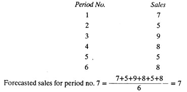
If our objective is the forecast or predict the sales of an item for the next sales period, then using this method,
Forecasted sales for next period = Average sales for previous period.
Example:
Technique # 9. Forecasting from Last Period’s Sales:
The method eliminates the influence of past (old) data and bases the forecast only upon the sales of the previous period.
ADVERTISEMENTS:
Using this technique, the forecasts would look as in table given below:
Technique # 10. Forecasting by Moving Average:
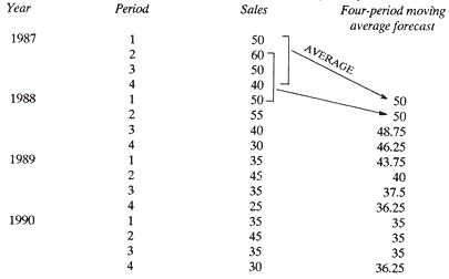
This method represents a compromise between the two above explained methods, in that the forecast is neither influenced by very old data nor does it solely reflect the figure of the previous period. Consider the historical sales figures shown in table below, which are to be used to construct a sales forecast for the next year. We must use a four-period moving average in this case.
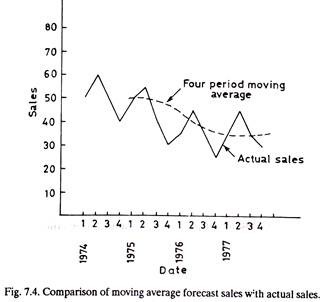
Fig. 7.4 shows that the effect of the moving average is to smooth the sales pattern and it is therefore of more value in establishing trends. The use of simple moving average is an adequate method of forecasting, provided sales are subject to neither seasonal variation nor marked secular trends. A secular trend is one which causes sales steadily to increase or decrease.
Technique # 11. Weighted Moving Average Method for Forecasting:
Whereas the simple moving average gave equal effects to each component of the moving average data base, a weighted moving average allows any weights to be placed on each element, providing, of course, that the sum of all weights equals one. As an example, suppose that in a four-month period the best forecast is derived by using 40% of the actual sales for the most recent month, 30% of two month ago, 20% of three months ago, and 10% of four months ago.
If actual sales experience was as follows:
The forecast for month 5 would be
F5 = 0.40 (95) + 0.30 (105) + 0.20 (90) + 0.10 (100) = 97.5
Suppose sales for month 5 actually turned out to be 110, then the forecast for month-6 would be:
F6 = 0.40 (110) + 0.30 (95) + 0.20 (105) + 0.10 (90) = 102.5
The weighted moving average method has a definite advantage in being able to vary the effects of past data, but it also has the disadvantage of remembering the total history for the time period.
Technique # 12. Forecasting by Exponential Smoothing:
The main disadvantages of the moving average method are:
ADVERTISEMENTS:
1. The lengthy calculations involved.
2. The need to keep quantities of historical data.
3. The fact that the normal (or simple) moving average method places equal weight on each of the historical figures used.
4. The age of the data, which increase with the number of periods used.
All of these disadvantages are overcome by the exponential smoothing technique.
Using this technique it is necessary only to retain the previous forecast figure and to know the latest actual sales figure. The technique works by modifying the old forecast in the light of new sales figure, i.e.
ADVERTISEMENTS:
New forecast = α (latest sales figure) + (1 -α) (old forecast)
where α is known as the smoothing constant.
For example, let
Forecast sales for last period = 24
Actual sales for last period = 22
Forecast sales for next period = α (22) + (1-α) 24
ADVERTISEMENTS:
Assuming α = 0.1
... Forecast sales for next period = 0.1 (22) + (0.9) 24 = 23.8
The use of this technique permits the forecast to respond to recent actual events, but at the same time retain a certain amount of stability. The amount by which the new forecast responds to the latest sales figure, or the extent to which it is damped by the previous forecast, is, of course, determined by the size of the smoothing constant α. The size of a should be carefully chosen in the light of the stability or variability of actual sales, and is normally from 0.1 to 0.3.
The smoothing constant, a, that gives the equivalent of an N-period moving average can be calculated as follows:
For example, if we wish to adopt an exponential smoothing technique equivalent to a nine-period moving average, can be found as follows:
When a secular trend is present, the forecast sales obtained by the normal exponential smoothing method will lag behind actual sales, in just the same way as the moving average forecast.
Econometric Forecasting:
In econometric forecasting the analyst tries to uncover the cause-and-effect relationship between sales and some other phenomena that are related to sales. For example, an appliance manufacturer might discover that the sales of television sets respond to the disposable income of customers with a 1-month lag. That is, 1 month after a change in disposable income, there a proportionate change in the sales of T.V. sets.
This process is called econometric forecasting. Here, the analyst tries to identify those factors that best explain the level of sales for a product. Econometric forecasting utilizes correlation and Regression techniques. The objective is to establish a cause-and-effect relationship between changes in the sales level of the product and a set of relevant explanatory variables.
Technique # 13. Correlation Analysis:
Correlation Analysis is frequently used if a relationship can be found between sales and other economic and non-economic phenomena, such as the national income, defense expenditures, population growth, and the weather. Such forecasts are generally concerned with the sales volume for the entire industry. The forecaster arrives at his company forecast by estimating the company’s share of total industry demand.
ADVERTISEMENTS:
One difficulty with correlation analysis is that a past relationship may not continue into the future. Correlation techniques are most reliable when a casual relationship can be established between the variables and sales. Correlation techniques have been used to develop demand functions for a number of products, such as furniture, refrigerators and automobiles.
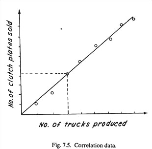
It makes use of cause-and-effect relationship between sales and some other phenomena that are related to sales. This technique is employed when an organisation finds that the sale of its product has a remarkable relationship with the sales of a leading product of another organisation, e.g., sales of clutch plates is correlated with the sales of trucks produced, (Fig. 7.5).
In correlation technique, total sales for an industry (e.g., truck manufacturing concern) is found and then based upon the market conditions, the volume of sale for one’s own product (e.g., clutch plates) is predicted. Such past data when plotted on the graph paper (refer Fig. 7.5) with line of best fit drawn, can predict sales estimate for future.
Sources of correlation data:
(i) Economic Data:
1. Survey of current business.
2. Monthly labour review.
3. Business magazines.
(ii) Industry Data:
1. Trade journals.
2. Annual survey of manufacturers.
3. Industrial trade associations.
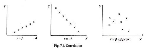
A Correlation Coefficient is a measure of the extent to which two variables (e.g. number of trucks sold and clutch plates sold) are associated. In other words, a correlation coefficient is an indication of the extent to which the knowledge of the value of one variable is useful to the prediction of the value of the other. This is the basis of a method of forecasting variously known as associative predictions or economic indicators.
Perhaps the most useful coefficient is the Pearson Product Moment Correlation Coefficient, which is calculated as follows:
Coefficient, r, for two variables x and y
Where x is the mean value of all the individual x values, and
y is the mean value of all the individual y values.
The formula measures linear correlation, i.e.
Example 1:
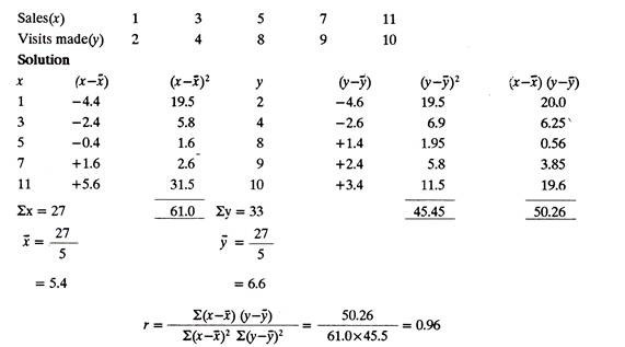
A comparison of monthly sales of an expensive item, against the total number of visits made by salesman during the previous month, yields the following data. Is the correlation of the two variables good enough to enable the number of sales visits, to be adopted as an efficient indicator of future sales?
The correlation between the number of salesman’s visits and the number of sales is 0.96, which is sufficient to justify its possible use as a method of short-term sales forecasting,
Technique # 14. Linear Regression Analysis:
Although computationally more difficult, this method is a very useful forecasting technique if past data appear to fall about a straight line. However, an estimate of how good the line fits the data is computed as part of the procedure. Forecasts of demand is related to economic and competitive factors which control or cause demand, through least squares regression equation.
The method is useful for short and medium range forecasting of existing products and services. Forecasting based on regression methods establishes a forecasting function called a regression equation. The regression equation expresses the series to be forecast, such as rupees sales or quantities sold, in terms of other series that presumably control the sales or cause them to increase or decrease.
An example of other series may be disposable personal income. If disposable income is up, sales will increase, and if people generally have less money to spend, sales will go down. The empirical relationship is established through the regression equation. It has been seen earlier that a linear relationship between two variables x and y is indicated by a high value of the correlation coefficient.
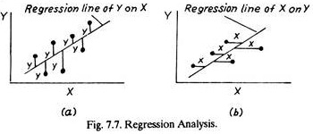
However, this coefficient does not indicate the true relationship, hence we are unable to estimate either a value of x for a given value of y or vice versa. To do this, a regression equation must be calculated (Fig. 7.7).
The regression line for Y on X is the best line for calculating values of Y, and is obtained by minimizing the sum of the squares of the errors of estimation, i.e. they values in Fig. 7.7(a) The regression line for X on Y is the best line for calculating values of X, and is obtained by minimizing the sum of the squares of the errors of estimation, i.e. the x values in Fig. 7.7(b)
The general equation for the regression line of Y and X is given by:
where a and b are two constant.
The values of these two constants are obtained by the following formula:
Similarly the general equation for the linear regression of X on Y is:
Example 2:
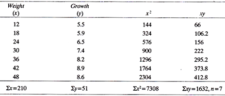
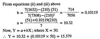
Given the data in table below, find the regression line for predicting growth and calculate the growth for a weight value of 50.
Let growth be variable Y
Let weight be variable X
... Y = a + bX
The regression line provides only an estimate of the value of Y on X. The uncertainty or accuracy of the estimate can be assessed by calculating the standard error of the estimate of Y on X, (SY.X)
where y = actual value
y1 = value calculated from regression equation.
The standard error of the estimate of X on Y is given similarly by:
SY.X or SY.X provides a measure of the closeness of the relationship between the two variables. The smaller the figure, the closer are the values to the regression line and hence the more accurate is the regression equation for predictive purposes.
